
Memo 0003: Calibrating a rooftop 21cm dual-channel spectrometer.
Canadian Centre for Experimental Radio Astronomy http://www.ccera.ca
Memo: 0003 Calibrating a rooftop 21cm dual-channel spectrometer.
To: Interested parties
Cc: Open Source Radio Telescopes
From: Marcus Leech, mleech@ripnet.com
Date: Oct 20, 2017
Subject: A process to remove the instrumental spectral response of a 21cm spectrometer.
This memorandum describes the process used at CCERA to calibrate the 21cm spectrometer, whose 2 1.2m dishes are situated on the roof of the CCERA lab building.
Astronomical Spectrometer Calibration
In an astronomical spectrometer, used to measure “interesting” astronomical emission lines like the 21cm line, the spectral peaks are usually no more than 2-3dB above the surrounding diffuse noise floor. In such an instrument, it is important to understand what the inherent spectral response of the instrument is, because, invariably, it will never be perfectly-flat at these fine power scales. Furthermore, the spectral artifacts introduced by the instrument can occur at similar scales to the astronomical phenomena that are being measured.
Various mechanisms contribute to a non-uniform instrumental response including:
- Inherent ripple of any analog filters
- Inherent ripple of any digital filtering processes
- Small-scale analog mismatches in cabling systems, leading to small standing waves and non-uniform spectral response
- Non-ideal behavior of ADCs and amplifiers
- Non-ideal FFT behavior
A process using “cold” sky
In an ideal situation, the antennae can simply be pointed at some “cold” spot in the sky where there will be nothing by uniformly distributed distributed noise created by non-line-emitting processes. The resulting spectral data are recorded, and then used in a later step to adjust the “live” data to remove instrument artifacts. Under such an ideal situation, any “lumps” in the spectral response of the instrument must necessarily be the result of instrumentation, and not attributable to any source within the response of the antennae.
In the case of the 21cm H1 line, finding such a spot in the sky, given a field-of-view of order 10 degrees, appears to be inordinately difficult. The whole sky is “alive” with hydrogen at some scale above background, contaminating any effort to use “cold sky” to measure instrument response.
A process using RF absorbent materials
Another approach is to place RF-absorbent materials in front of the dish feed, to remove the sky signal completely, leaving just the instrumental response. In an ideal situation, the absorbent material will present a completely-uniform black-body spectrum to the instrument, with a blackbody temperature close to the ambient temperature of the material.
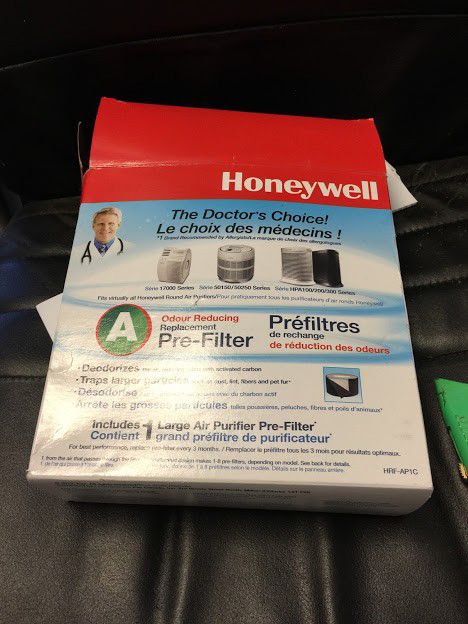
This intrepid experimenter made an attempt to use a carbon-filled fabric, as is used to provide pre-filtering and odor-removal for residential HEPA air cleaners. Shown below is a package of the material we had lying around in the CCERA lab:
How RF-absorbent are pre-filter materials?
The material can be cut with easily with scissors. It was decided to mount three layers of this material on a coroplast backing of 25cm diameter, which matches the diameter of the feed-cone aperture on our 21cm feeds.
We had no notion of exactly what the attenuation capabilities of this material would be, but decided that since it contained chunks of carbon, it would be a suitable material for the experiment.
Two such three-layer “pads” of the material were constructed and applied to the mouth of the feeds, held on with painters tape.
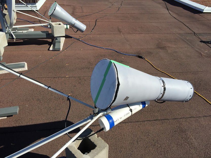
The 21cm feed horns “gagged” with pre-filter material.
Returning to the laboratory from an excursion to the roof, and waiting several minutes for data to be collected and averaged, we fully-expected to find a nice, uniform spectrum, without any hint of the hydrogen line. We were spectacularly disappointed. While careful inspection of the raw data indicated that the stack of carbon fabric had offered about 0.5dB of attenuation, that was clearly insufficient to “wash out” the H1 spectral response. It appeared in the data, robustly. It is a testament to the sensitivity of both the electronics of these systems, and the power of the signal processing and back-end data processing afforded by modern computing environments.
Clearly, this approach requires purpose-manufactured RF absorbent foam, and not ad-hoc cm-scale few layers of a vaguely-similar material. We briefly considered trying the same experiment with a healthy bag of activated carbon in front of the feed, but opted for a different approach.
A process using the ground, or its reasonable proxy, the roof
Dry ground makes an excellent black-body source, emitting as a black-body with an equivalent temperature close to the ambient temperature of the top layer of soil, proportional to the wavelength. Such a source will have a uniform, smooth spectral distribution, and at fractional bandwidths as small as the ones used in hydrogen-line spectroscopy, perfectly flat.
Our dish antennae (and their feeds) are situated on a roof, approximately 8.5m from the ground. However, the roof surface itself should also make an excellent black-body emitter, being made from reinforced poured concrete, roughly 50cm thick, topped with gravel and bitumen cloth.
We opted to simply dismount the feeds temporarily, and situated them aperture-down onto the roof surface.
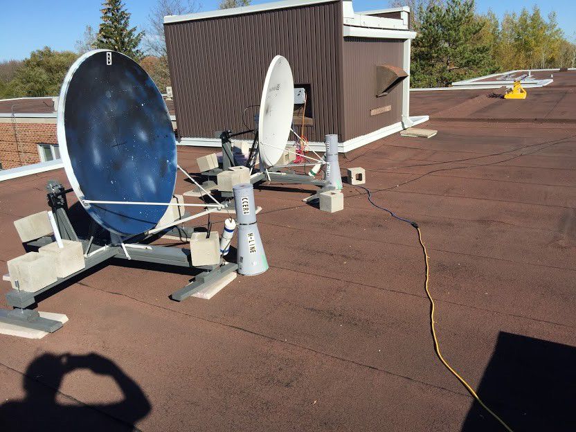
The feed horns were dismounted for calibration.
The process of dismounting took only a few minutes, and the feeds were quite stable in that configuration, despite the considerable breeze “up top”.
We retreated back to the ground-floor lab, and waited for the integrator to converge. Once a few minutes had passed, we inspected the semi-raw data, and found what we were hoping to find:
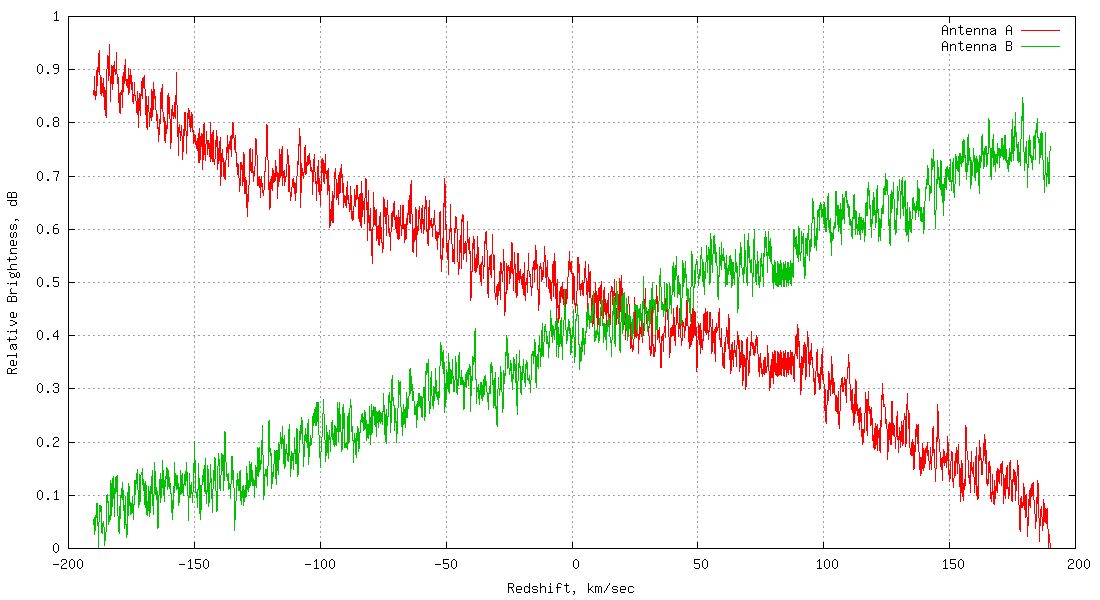
“Dark frame” calibration data from the dismounted horn feeds to be used to normalize observational data.
This data was exactly what we were looking for. We already knew that there was a distinct slope in the response for both channels, and there is some evidence of a regular, but small, ripple in the above data. Coincidentally the nature and sign of the slope was somewhat different for both channels. The first-stage filters are very broad (about 200MHz), and likely have pass-band ripple of order 1dB. The two filters won’t have ripple components in precisely the same places, so a different slope response over what amounts to 1.25% of the total filter bandwidth is not a surprise. If one then considers other components in the system that may have non-uniform gain response, then fine-scale differences in overall instrument response seem inevitable.
This data, then, could be used as a “dark slide” to subtract-out the instrument response from the live sky data.
Data processing
In an astronomical spectrometer, one is concerned about the spectrum of the emissions coming from the sky, and not necessarily about the total, absolute, brightness integrated over the entire pass-band of the instrument.
It is useful to take advantage of this fact, and routinely normalize or “baseline” the spectral data so that it is always relative to some zero point. You can see in the plot given above, that everything is in dB, relative to zero dB. This is useful, for example, when subtracting calibration spectral data that have been derived from a black-body source that may be at an absolute temperature/brightness significantly higher than the sky signals. Applying this technique to the spectral data also ameliorates the significant tendency of sensitive radio telescopes to undergo gain changes during their operation, due to temperature fluctuations. One simply hopes that those gain fluctuations do not also result in significant fluctuations in the spectral response of the instrument. It is likely, however, that at fine scales, the spectral response of the instrument also changes with temperature fluctuations. One does what is practical, and shrugs ones shoulders about the rest.
It should be noted that this technique would be unacceptable for a continuum radiometer, but provides analysis benefits for a spectrometer. A continuum radiometer inherently measures the total power across the analysis bandwidth, where the “baseline noise” is what it is actually measuring—continuously “normalizing” that baseline to zero would remove the data one is trying to collect.
Extracting brightness temperature from normalized data
It is useful to remember that the detector of a radio telescope has an output, D, proportional to:
D ~ G(Tsys + Tsky)
In this case G is the system gain, Tsys is the total system noise temperature (composed of several component sources), and Tsky is the noise temperature due to the sky within the field-of-view of the antenna.
If one has a reasonable estimate for Tsys and some notion of what Tsky should be in any given pointing situation, then simple algebra can be used to determine the brightness estimate for any given spectral component. For “sloppy” fields of view typical of an amateur scale instrument, the diffuse Tsky at 21cm (absent spectral contributions from H1) will range somewhere between 10K and 20K.
Using all the above, we can produce “pretty” plots showing brightness estimates, such as given below.
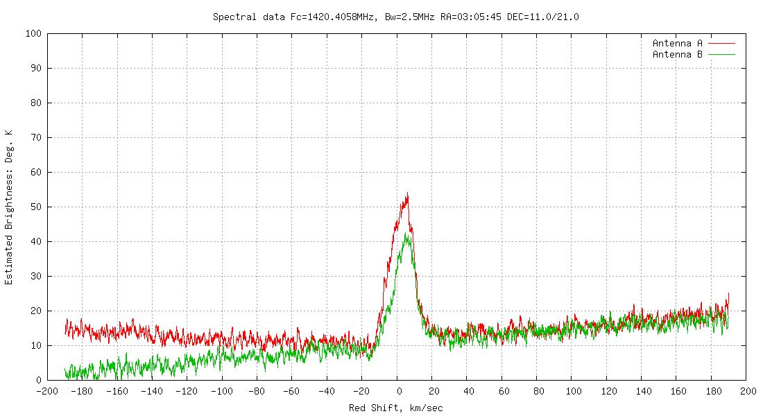
Observed brightness after subtraction of the “dark frame” background data.
Frequency calibration
This memo has not dealt with the subject of frequency calibration, which is important in deriving precise Doppler velocity estimates from spectral data. It is the case that the spectrometer at CCERA has a reference clock that is accurate to approximately 5PPB. This translates to an uncertainty in Doppler velocity of roughly 0.1 cm/sec at 200 km/sec velocity—the extreme of Doppler velocities expected from within the galaxy.
It is relatively easy, even for the amateur observer, to use excellent-quality reference clocks for SDR receivers, removing the need for tricky frequency calibrations against borrowed sources, or shortwave-broadcast time standards. A GPS-derived 10MHz reference, which easily provides 5PPB or better accuracy, can be acquired for under $200.00 in the current market.
More exotic options, like Rubidium clocks are also an option, and not much more expensive than a GPS reference clock, providing sub-1PPB accuracy.
Lower on the cost scale are oven-controlled crystal oscillators (OCXOs). These provide accuracy of approximately 20-50PPB after warm-up, and can be purchased on the surplus market for approximately $20-$30 each.
Conclusions
We used a simple, ad-hoc, black-body source to calibrate the spectral response of an astronomical spectrometer.
Simple numerical methods were used to derive useful scientific measurements from the post-calibration data.