
Memo 0006: A precision hydrogen spectrometer based on AirSpy receivers
Canadian Centre for Experimental Radio Astronomy http://www.ccera.ca
Memo: 0006 A precision hydrogen spectrometer based on AirSpy receivers
To: Interested parties
Cc: Open Source Radio Telescopes
From: Marcus Leech, mleech@ripnet.com
Date: Nov 13, 2017
Subject: AirSpy Receivers for hydrogen line spectroscopy
This memorandum describes the design of a precision spectrometer receiver based on AirSpy SDR receivers and supporting auxiliary hardware and software.
Hydrogen Line Spectroscopy
The hydrogen line, with a rest frequency of 1420.4057517662 MHz (21.11cm) occupies a special place in the menagerie emissions from the Cosmos. Interstellar space is “full” of neutral hydrogen, which occasionally undergoes a hyper-fine transition of the electron spin, producing a single photon at 21.11cm. The spatial density of this hydrogen is low—an atom or two per cubic meter. The temporal density is also low—perhaps 1 event per 1e5 to 1e6 years. But along any given line of site, there are a tremendous number of these hydrogen atoms.
Since interstellar hydrogen is ubiquitous, most of it can be easily detected by a small-scale observatory, with modest equipment.
Mapping the spatial distribution of hydrogen across the sky, along with the apparent frequency shifts caused by Doppler effect, allows the dedicated observer to calculate the rotation-curve of our galaxy.
Antique Analog Spectrometers
In a “traditional” (or, realistically, antique) spectrometer, signal frequency components are extracted by sweeping a narrow-band receiver through a frequency range, with a power detector connected to the back of the receiver. The current frequency and power-levels are recorded, producing a spectral estimate across the sweep frequency range.
FFT Digital Spectrometers
In modern receiving systems for radio astronomy, the bandwidth of interest is digitized prior to any further manipulations being performed on the signal bandwidth. What this means is that it is easy to use Fourier Analysis on the signal to extract the frequency components of that signal.
In our case, we digitize the signal bandwidth (2.5MHz centered on the hydrogen-line reset frequency) using an AirSpy SDR-based receiver, and use the Gnu Radio toolkit to process the signal through a Fast Fourier Transform (FFT) function.
The Gnu Radio flow-graph is shown below:
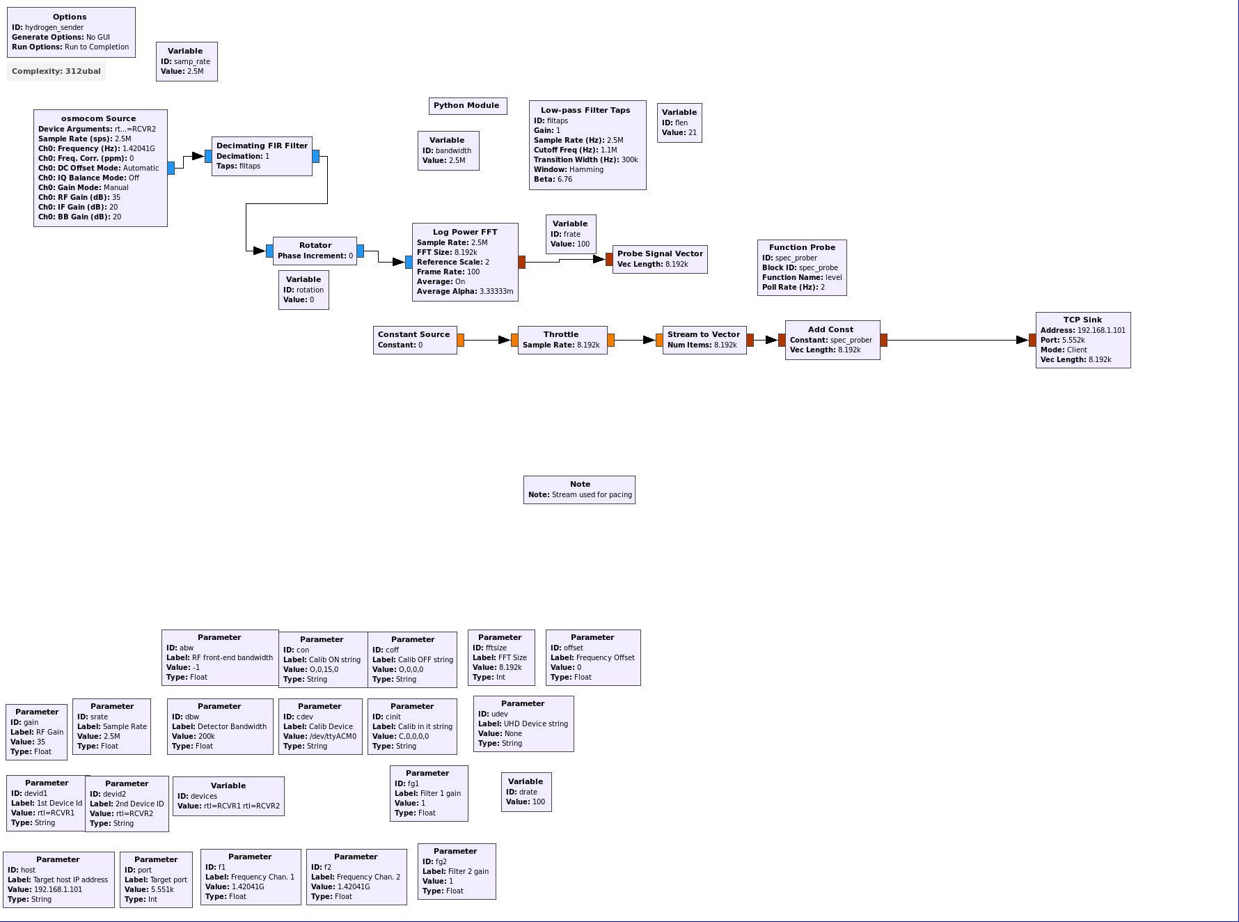
GnuRadio Flow-graph for Spectrometry
Main flow-graph elements
Osmocom Source
The source block is unremarkable—in our case, it is configured to operate at 10Msps, using an AirSpy input device.
Decimating FIR Filter
This block consumes the 10Msps input from the AirSpy and filters and decimates the signal to 2.5Msps, providing roughly 2.2MHz of usable bandwidth.
Rotator
This block is used to provide fine frequency adjustment. This is necessary to ensure that the central frequency is “exact”, as synthesizers generally have a small-but-finite frequency precision. In more advanced SDRs, the precision of the synthesizer is accounted for in FPGAbased DSP code, but AirSpy has very little “on board” DSP functionality.
Log Power FFT
This block, as its name suggests, computes a FFT of the input signal, then computes the magnitude -squared (thus, power) component, and then converts into dB form. It also performs averaging, via a simple single-pole-IIR function.
The block is configurable with respect to FFT size (we tend to use 8192 bins), alpha value for the single-pole-IIR computation, and a so-called frame rate. This rate is the rate at which FFT computations are performed over the incoming time-domain sample stream. In an ideal situation, the frame rate simply be sample-rate/number-of-bins. But in our case, due to our computing architecture, we cannot quite compute FFTs in “real time”. Instead, we use a framerate that is approximately 1/3rd of “real time”, and then use averaging to make up for the loss in sensitivity that results.
Probe Signal Vector
The vector of dB values from the FFT is “terminated” in a probe block. This block can be “probed” at a leisurely pace and then logged locally, or sent via TCP to a “gatherer” computer.
Data-dumper secondary flow
The rest of the flow-graph involves extracting data from the “probe” and sending it via TCP to a central computer where it is further integrated, tagged, and logged. This data is sent at a rate of approximately 2Hz, and the “logger” integrates and dumps every 90 seconds.
Potential Sources of Error
An astronomical spectrometer measures two quantities—the Doppler shift (as represented by a frequency offset), and the brightness.
Both of these quantities are subject to instrumental inaccuracies and systematic error.
Fixed Frequency Offset Error
It is the case that no electronic oscillator is “perfect”, and those found in radio receivers are no exception. The frequency synthesizers that are used in modern SDR receivers have a small-butfinite tuning precision. In the case of the AirSpy, at the hydrogen-line rest frequency, that resulting “imprecision” means that the synthesizer in the tuner is “off” by 20Hz. We compensate for that fixed offset by including the Rotator block in the flow-graph above. AT the hydrogen line frequency, a 20Hz offset means a Doppler velocity error of 4.2m/sec. This is very small, but since we have the means to compensate cheaply, we do so.
Frequency Uncertainty Error
Frequency synthesizers require a reference clock in order to produce the final frequency that is used to down-convert the “sky” frequency to baseband. The AirSpy has an internal reference clock with a frequency uncertainty of approximately 5.0e-7 Hz, which is about 710Hz at the line frequency, or approximately 149m/sec represented as a doppler uncertainty.
Many SDRs include the ability to use an external reference clock, usually at 10MHz. The AirSpy supports an external 10Mhz clock with an amplitude of no greater than 3.3V. The CCERA spectrometer can select among 3 different clock-sources that are external to the AirSpy:
- An insulated, oven-controlled, crystal oscillator, giving 2.0e-8 frequency uncertainty.
- A GPS disciplined oscillator, giving, 1.0e-10 frequency uncertainty.
- A Rubidum-cell 10MHz reference, giving 1.0e-11 frequency uncertainty.
It is interesting to note with a frequency uncertainty of 1.0e-11, Doppler measurements down to 0.3cm/sec could, in a spherical cow sense, be achieved.
Passband Spectral Response Uncertainty
Any real-world receiver system will have a non-uniform magnitude response across its passband. Such non-uniformity will be the convolution of the individual responses of system components.
There are two main types of such non-uniform response that contribute to uncertainty about spectral features extracted from the data samples. One of which is pass-band slope, and the other is pass-band ripple. Slope across the pass-band can often be as much as 1dB, while ripple is usually on the order of 0.1 to 0.2dB. The magnitude of these components is easily large enough to provide sources of uncertainty and ambiguity in spectral measurements whose “real” features are barely larger than the inherent instrument response.
The mechanism that we use at CCERA to deal with these is to use a “dark slide” consisting of several layers of carbon-filled foam that are placed in front of the feeds while measurements of the system response are taken. The carbon-foam acts as a uniform noise source so that any nonuniform response is due entirely to the instrumentation.
Once that data is available, it can be used as part of a “normalization” process to good-quality spectral estimates from the raw FFT data.
Linearity Errors
Analog radio receiver systems are known to have operating regions where they operate in a largely-linear fashion, and regions where they don’t. There are many factors that contribute to this, including mixers, amplifiers, ADCs, filters, switches, etc.
A useful approach is to eliminate, where possible, those situations where non-linearity can creep into the system. A useful first approach is to ensure that the RF chain is rigorously filtered as early as possible in the receive chain, and that filtering is repeated throughout. In our design, we filter between the first two LNA stages, and again right in front of the receiver. Additionally, the feed structure itself (a circular wave-guide) affords significant filtering below the cur-off frequency of approximately 1.1GHz. Filtering so that most of your system only ever “sees” the quite-weak astronomical sources in the sky means that it is unlikely to enter into the non-linear regions of amplifier operation.
Further, we adjust our gain so that the ambient sky noise “fills” about 70% of the available ADC bits. This gives adequate headroom to assure linear operation of the ADC, while maximizing sensitivity given the above constraint.
Radio Frequency Interference
Radio frequency interference, or RFI, is a constant and growing concern. The hydrogen-line band, from 1420 to 1427 MHz is notionally “reserved” for radio astronomy, but in practice can sometimes be contaminated with unintended signals. Is is frequently the case that such signals originate within the radio telescope instrumentation itself.
The hydrogen-line spectrometer suffers from a strong “spur” at exactly 1420MHz, created by the 10MHz clock circuitry producing the 142nd harmonic. We simply delete-and-smooth that narrow-band “spur” in post-processing.
Brightness Estimate Uncertainty
For rotation-curve studies, the absolute brightness of the hydrogen-line spectral features is not that important compared with the doppler-velocity estimates.
However, for purposes of making high-information-content maps, the ability to derive a consistent brightness estimate is exceedingly useful.
Several factors contribute to uncertainty involving the magnitude of spectral features, and how they relate to apparent sky brightness.
In any radio receiver system, the overall system gain, and apparent noise temperature will vary with time. This time-varying property is most strongly coupled to the ambient temperature of the various gain-related components in the system, but other factors such as temperature changes in the antenna spill-over regions, noise in the antenna sidelobes, etc, also play a role.
One approach to this problem with spectral data is to make several simplifying assumptions, in order to derive a very-crude sky-brightness estimate.
If one assumes that system noise temperature, Tsys, remains within some small bounds, and that gain remains within some small bounds, then one can produce a crude estimate by observing that:
P ~= G(Tsys+Tsky)
If we have a rough estimate for Tsys, and we assume that Tsky for the “baseline” portions of the spectral estimate is fixed within the range of perhaps 15-20K (which is reasonable at 21cm), then it is a simple matter of algebra to convert “normalized” (baseline-subtracted) spectral estimates into brightness estimates. A modification of this approach would be to consult online sky maps for Tsky estimates near 21cm (perhaps at 1415MHz), and use that data to set Tsky for any given measurement at a given RA/DEC in the data. But in a sense, that feels like “cheating”.
A better method, and one which CCERA is working towards, is to use a routine calibration procedure. In our case, that will consist of electronically switching the entire receive chain after the feed between the feed, and a temperature-controlled termination. If one switches the receiver chain to a controlled load on a regular basis (a few times per day), it allows for good-quality calibration of the instrument. In the case of CCERA, the terminator will be maintained at 340K at all times, along with the two-stage LNA. This both provides a terminator with a known blackbody equivalent temperature, and stabilizes the temperature, and thus gain and noise-figure of the LNA.
What this means is that there will always be “fresh” dark-slide data, and that data will represent a noise source with a fixed, stable, black-body temperature of 340K. A previous memorandum in this series described the so-called “thermal stage” we use to achieve this.
FFT Resolution
The FFT resolution directly determines the Doppler velocity resolution provided by the system. In the current configuration, we use an FFT resolution of 8192 bins, which amounts to a binwidth of approximately 305Hz, or 64m/sec.
If it is desired to achieve higher Doppler velocity resolution (commensurate with the underlying frequency uncertainties previously discussed), then using a larger number of FFT bins is easily achievable at the expense of more disk storage space.
System Design
Shown below is a high-level diagram of the spectrometer system:
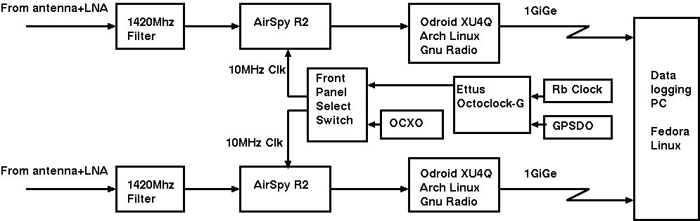
High-level schematic layout for the Spectrometer
The receiver cabinet is shown in the image below.
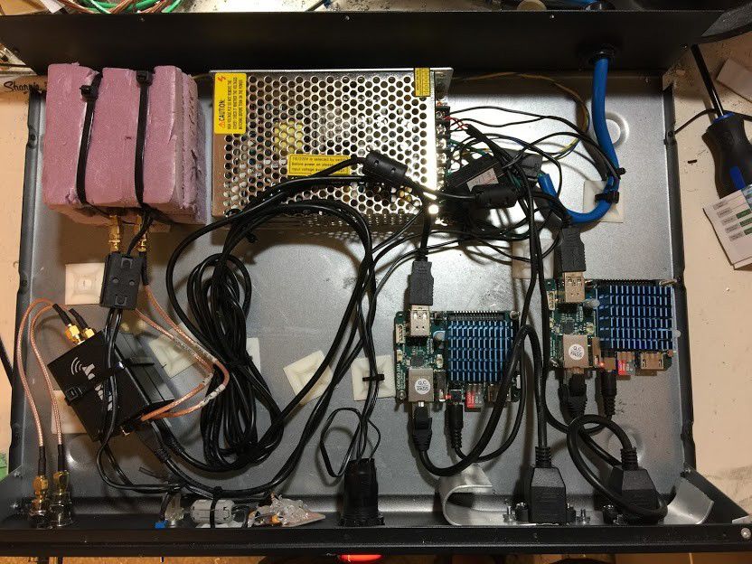
The Receiver Cabinet
Of note are the AirSpy receivers in the bottom-left, the Odroid single-board computers, shown with blue heat-sinks, and the 10MHz ovenized oscillator, surrounded by pink high-density styrofoam. The final filters are located outside the receiver cabinet, to allow easy experimental reconfiguration for other projects.
The power-supply provides +12VDC for the ovenized oscillator, and +5VDC for the Odroid single-board computers and AirSpy receivers.
Typical Results
Here we show a snapshot of the hydrogen spectrum in the Cygnus region.
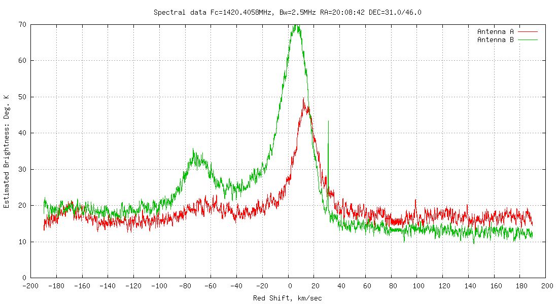
Sample spectrum: Cygnus Region
Conclusions
We show a system design that is capable of producing high-quality spectral estimates for the 21cm hydrogen line. In the future, we will be able to improve brightness estimates considerably using techniques discussed in this memorandum.