Memo 0012: A pulsar observing capability at CCERA

To:Interested parties
Cc: Open Source Radio Telescopes
From:Marcus Leech, patchvonbraun@gmail.com
Date:Oct 14, 2020

Subject: A pulsar observing capability at CCERA

This memorandum describes the equipment and techniques used to engage in routine monitoring of bright pulsars, in particular, J0332+5434.

Acknowledgements

The work described herein could in no way be considered entirely novel. It is the product two years of protracted effort with useful input from dozens of people. The work could not have proceeded without the suggestions, criticisms, occasional rancor, and code snippets from the dedicated and skilled observers who are denizens of the neutron-star mailing list1 and associated website.I am indebted also to Daniel Marlow at Princeton, who agreed to test versions of this system on the TLM-18 dish at the InfoAge in New Jersey. The staff and scientists at the SETI Institute and the Allen Telescope Array, in Northern California—their donation of weekend telescope time was vital in ironing-out bugs and tuning software features. Helpful pointers from Wael Farah at the ATA contributed to a better understanding of the finer-points of epoch folding in pulsar observations.

Pulsars

Much information is available on the detailed physics of pulsars—that information will not be repeated here. But a quick precis will be useful in understanding the challenges involved in performing observations with modest instrumentation.

Pulsars are the highly-magnetized remnants of stellar collapse for stars within certain sizes ranges. These stars collapse into a Neutron Star which in many instances gives rise to a pulsar. Two details in this collapse process are important to understand. Firstly the original angular momentum of the star is preserved across the collapse—this inevitably means that the resulting collapsed star will begin spinning at a considerable rate. Neutron stars begin life as large stars, and when they collapse, they collapse into highly-condensed matter with a diameter usually no greater than a small city here on earth. The original magnetic field of the star also collapses, which again means that it has considerable density after collapse.

It is this strong magnetic field that is thought to be responsible for the radio pulses seen on earth as pulsars. Synchrotron emissions emerge along the two magnetic poles of the neutron star, and due to the rapid rotation, and the typical offset of the magnetic poles from the axis of rotation, a “lighthouse” effect is produced. When one of the “lighthouse” beams sweeps past earth, we see a broadband radio “pulse” as it sweeps past.

These pulses are very weak compared to other types of cosmic sources that may be familiar to the small-scale radio astronomy observer. The brightest pulsar in the northern sky is J0332+5434 with a mean pulse brightness at 408MHz (our observing frequency) of only 1.5Jy. In dramatic contrast, Cygnus A has a brightness at 408Mhz of 4800Jy. A further complication and challenge is that the duty-cycle for a typical pulsar is quite small. For J0332+54, the pulse-width is 0.0066s with a pulse period of 0.714520s, giving a duty-cycle of less than 1%. Those “lighthouse” beams are sweeping past earth with much haste, and as they do so, they deposit very little energy into our antennae.

The RF energy from a pulsar source is, like many cosmic sources, very broad-band in nature. Because pulsar sources are inherently synchrotron sources they produce more energy at longer wavelengths (lower frequencies) than at shorter wavelengths, which prompts amateur and small-scale observers to focus their efforts on the lower frequencies. Because of the somewhat-steep spectral index of most pulsars, the brightness difference can be dramatic. The pulsar we discuss here, J0332+5434 has a spectral index of 2.4. This results in the brightness at 611Mhz being 2.63 times smaller than at 408MHz. Thus the 408Mhz mean brightness of 1.5Jy becomes only 0.570Jy at 611Mhz. Observing at lower frequencies comes at a price, however. Due to the dispersive nature of the interstellar medium (the ISM), the pulses at higher frequencies (shorter wavelengths) will arrive slightly before the pulses from the lower frequencies (longer wavelengths). In practical terms, this means that without taking that effect into account, the pulses can become smeared in time–often to levels that completely preclude successful observation.

Observing Strategy

In conventional continuum-type radio astronomy we seek to maximize a number of system parameters to improve our observation sensitivity:

• Antenna aperture
• Receiver/observing bandwidth
• Integration time
• Minimize system noise temperature (Tsys)

Pulsar astronomy adds another performance dimension

• Sampling clock quality

A typical small-scale effort is limited in all of those dimensions. Observing bandwidth is limited Page 2 of 13primarily and typically by RFI considerations, but constraints on budget are also a consideration. It is typically the case that antenna aperture is constrained by budget and site considerations and system noise temperature is (the lower the better) is limited somewhat by budget—although modern low-noise-amplifiers that are more than adequate for routine pulsar observations are routinely available cheaply. Cryogenics are still an area where amateur and small-scale observers have neither the budget nor the expertise.

Integration time is sometimes limited by the type of antenna structure that is used. A transit-type instrument (such as we use at CCERA) limits the observing time during a single day. A tracking antenna affords much longer single-session integration times.

Clock quality is constrained largely by budget, and having a reference clock of reasonable stability and accuracy can be the “difference that makes a difference” in observing pulsars.

De-dispersion

We had previously discussed the notion that pulses from the source pulsar are dispersed by the ISM—the exceedingly-thin plasma that exists in inter-stellar space. The lower frequencies take longer to propagate through that medium than the higher frequencies. Given any non-trivial observing bandwidth, particularly at lower observing frequencies dispersion across the observing bandwidth of 10s of milliseconds is not uncommon. For our own observing set-up the dispersion at 408MHz over 5Mhz of bandwidth for the J0332+5434 pulsar is almost 17 milliseconds—recall that our pulse width for that pulsar is only 6.6 milliseconds. This means that without some type of de-dispersion strategy, the pulses will be smeared below the detection threshold in a typical case.

In pulsar astronomy there are two strategies for coping with dispersion. The main strategy for “real-time” observations is based on the observation that small amounts of residual smearing will not unduly affect the final SNR. This technique, known as incoherent de-dispersion breaks up the incoming bandwidth into a number of discrete sub-bands (a so-called filterbank), with each of the sub-bands being detected separately. The detected sub-band/filter-bank outputs are then added together through a set of delays in order to have the pulses arrive at the “adder” at more-or- less the same time, thus mostly eliminating the smearing effect from ISM dispersion. This technique has been in use for many decades, beginning in the all-analog era of radio astronomy observations and continuing to this day in the era of DSP and SDRs.

Another approach, originally devised by Hankins and Rickett in 1973, seeks to completely model the ISM dispersion as a transfer function whose properties are based on the measured Dispersion Measure (DM) of the source pulsar signals as they traverse the ISM. Once the transfer function is understood, it is easy to construct a specialized digital filter to completely “invert” this transfer function and completely and accurately remove the effects of dispersion. Such a digital filter is usually based on the Fast Fourier Transform and the filters that can be constructed from an FFT implementation. Such a filter has high computational complexity and yields filters that are very compute-intensive to realize. It is not usually the case that coherent de-dispersion is used in real-time observing, and it is prohibitive for most amateur and small-scale observers to contemplate.

Our own observing “pipeline” uses incoherent (delay-based) de-dispersion exclusively. Indeed this author is aware of only a single amateur/small-scale pulsar observer using coherent de-dispersion. It is of little advantage for the types of relatively-bright pulsars that amateurs are likely to attempt observations of. Our filter-bank implementation uses a simple windowed FFT channel-former with a modest FFT size—this makes it computationally unobtrusive.

Epoch Folding

The “tail end” of a pulsar observing chain is usually a so-called epoch folder. This technique is also known as synchronous detection. It takes advantage of known periodic behavior in the incoming “signal” to effect detection and enhance the Signal-to-Noise Ratio (SNR). Recall that pulsar signals are very-reliably periodic (indeed, as clock-sources, many pulsars would rival the absolute-best clocks we can produce here on earth), and that they produce narrow pulses. Recall also that they are exceedingly-dim sources. It is not uncommon for a pulsar signal to be hundreds to thousands of times weaker, as seen by the antenna feed, than the inherent system noise in the observing system.

Recall from statistics that the variance of uniformly distributed noise decreases with the square-root of the number of samples. The more samples you take (through virtue of both observing time and observing bandwidth), the faster the noise will “settle” into a steady, fixed level, with very little variance. If we arrange for our samples to be carefully “binned” so that they span exactly one pulsar period, then the pulsar pulses will be constantly added to the same bin in our exactly-one-period set of samples. This means that over time the pulses will add linearly, and the random noise will decrease proportional to the square-root of the observing time. This is the essence of an epoch folder, so called because the samples are “folded back” over the pulsar period, encouraging the (exceedingly-weak) pulses to slowly add in a linear fashion.

It is in this so-called epoch folder that clock quality becomes important. The system clock must be stable and accurate, in order to provide a predictable and stable sample-rate going into the epoch folder. If the clock drifts and/or isn’t accurate then the sample-rate will suffer accordingly. The pulsar pulses will “drift” over the time/phase bins, and sensitivity will be reduced—often catastrophically.

Instrument Hardware

Antenna and Feed

Our equipment choices have been largely dictated by our observing goals—we wish to observe J0332+5434 on a daily basis to provide data to a local university for their undergraduate-level course in astrophysics. The target pulsar is “bright” at lower frequencies, which means that an antenna with quite-modest gain is required to observe it. Indeed many amateurs now routinely observe J0332+5434 with a more-modest antenna than we use at CCERA. Our antenna, is a 3m mesh parabolic reflector, with a full-wave loop feed. It provides more than enough antenna area to realize our observing goal.

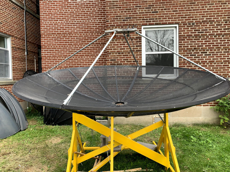
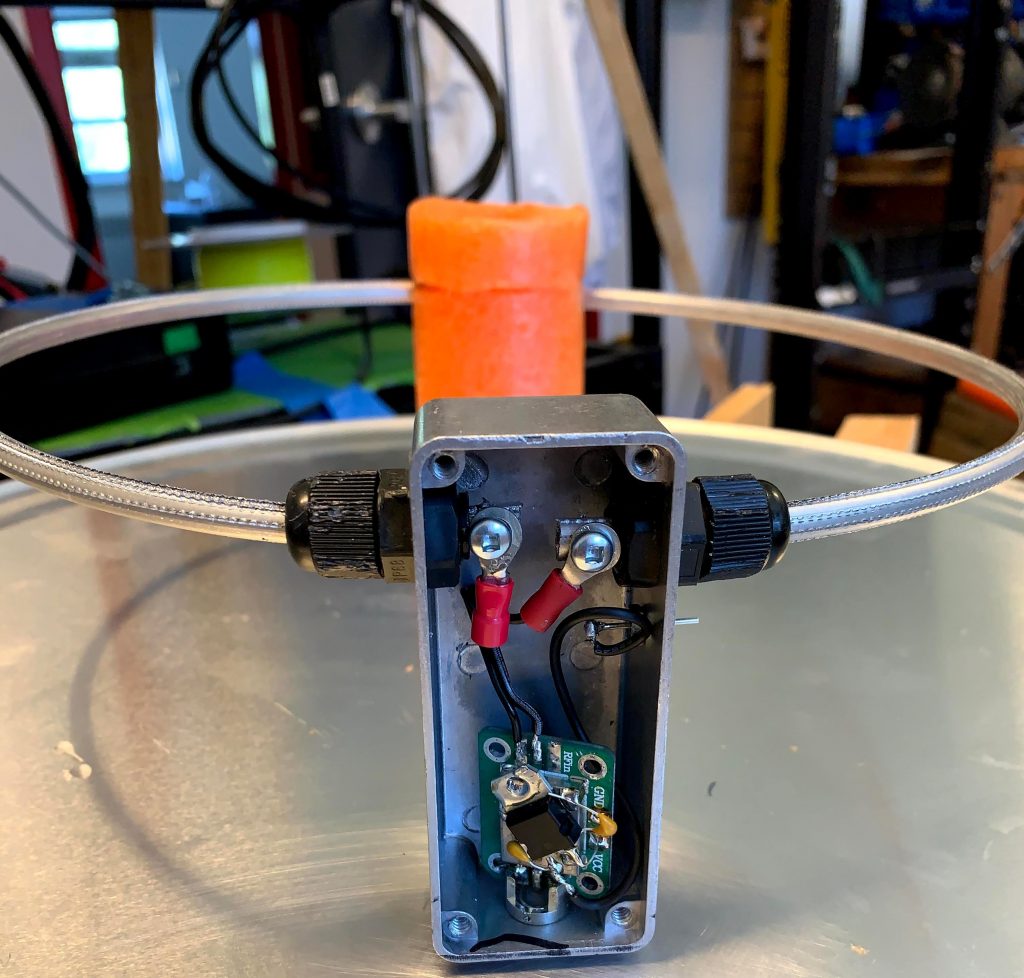
The feed shown has an integral low-noise amplifier, based on the SPF-5189Z MMIC LNA IC. It provides roughly 23dB of gain, with a noise figure of roughly 0.4dB (roughly 28K noise temperature). This connects to a secondary assembly beneath the dish with filters and line amplifiers to drive our 70-meters of feed cable between the dish and the receiver assembly.

The feed provides good illumination for our F/D = 0.4 dish, and has a feed-point impedance of about 60 ohms (VSWR 1.2:1).

The dish mount provides a fixed pointing—we can only make pulsar observations when J0332+5434 transits our local meridian, providing approximately 1.5 hours of useful observing time each day.

Receiver hardware

Our current receiver is a USRP B210 Software-Defined Radio receiver made by National Instruments under their Ettus Research 4 brand. We use only one of its two mutually-coherent input channels at this time, but may upgrade to a dual-polarization feed scheme, which would require use of both input channels.

Reference Clock

The receiver is connected to a reference clock that provides a higher-quality clock signal than can be produced internally in the SDR receiver, although the internal clock is good enough for short observing sessions, our laboratory has a rubidium atomic clock that offers frequency stability to
better than 0.01PPB (1.0e-9). Ours is a surplus model FE5680 set for 10MHz output—as required by many radios that take an external reference input. Such rubidium frequency standards are routinely available on the surplus market for under U$200.00 each.

Computer Hardware

The computational requirements of our pulsar software aren’t particularly strenuous at 5MHz observing bandwidth. Most modern desktop-class computers can easily handle the processing load. We happen to have an AMD Phenom II X6 that performs “management” functions for many of our ongoing observations, and currently the pulsar receiving chain operates on that computer.

It will work acceptably well on any of the higher-end ARM-based SBCs as well, including the Odroid XU4, and likely the new Raspberry Pi4 systems.

Software

All of the radio astronomy signal processing at CCERA is based on the Gnu Radio 5 software DSP platform. The pulsar signal-processing chain is no different.

We have developed a Gnu Radio application, called stupid_simple_pulsar 6 that provides the entirety of the real-time components of our pulsar processing setup. It is available on the CCERA github repository: https://www.github.com/ccera-astro. The name of the software is,
unfortunately, increasingly inaccurate, as it contains considerable sophistication and commensurate complexity. The Gnu Radio framework allows one to develop quite sophisticated signal-processing chains quite quickly, which means that ideas grow from simple to somewhat-
complex quite quickly.

The following flow-graph shows the top-level signal flow involved.

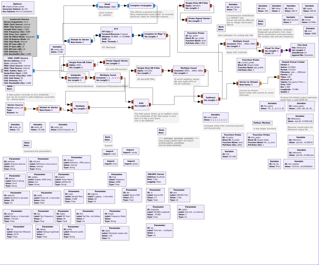
It looks quite daunting but it should be noted that a lot of the blocks are simply command-line parameter blocks which play no direct role in the signal flow, although they necessarily strongly suggest some of the underlying sophistication.

[It may be best to follow-along by bringing stupid_simple_folder.grc into GRC on your system to make it clearer how the signal flows]

Basics

The signal arrives at one of two “source” blocks—the build script builds a version both for osmosdr-supported devices (RTLSDRs, AirSpy etc) as well as a UHD-only version that allows access to some of the USRP-only capabilities.

The signal then proceeds to a head block that simply governs how long the script will run for— the block controls how many samples will pass through it before it declares itself (and thus allthat followd) “done”. The signal undergoes a spectral inversion with a complex-conjugate block, which is done simply to make some of the other processing more convenient—both for internal blocks and external pulsar processing tools, such as PSRCHIVE, SIGPROC, DSPSR, etc.

Filterbank Conversion

The signal then proceeds to an FFT block whose sole purpose is to provide a (some would say crude) filter-bank function. The FFT output is converted into a power estimate by virtue of a complex-to-mag2 block, and it is then integrated and decimated with an integrate block. Once it is in this form, each channel is operating at a lower sample-rate than the incoming sample rate. Typically the graph is configured (via command-line options) for a sample rate of 2-4ksps per channel. The higher the decimation value in the integrator block, the lower the output rate of the filter-bank. The output of the integrator goes both to a probe block, via a simple low-pass filter
and also to a multiply-constant block. This block serves to provide an RFI-removal and passband-smoothing function that will be described later. The output of this goes to an add block that serves to add-in the output of a pulsar simulator, that is disabled by default, and will be discussed later. The signal then enters a high-pass (DC block) filter that is implemented with a
signal branch that goes to a low-pass filter with a low corner frequency (a fraction of a Hz). The output of this low-pass filter is then subtracted from the main signal branch, which effects an inexpensive high-pass function. The net effect is to subtract-out the average DC level from the signal, leaving only the higher-frequency components, including our pulses and the attendant high-frequency system and external noise.

The signal then branches again—one branch going to a subsystem to create a standard filterbank file, the other to a custom block that implements an epoch folder. Up until this point, the signal has been in a vector format—with a vector size that is the same as the number of channels in the filter-bank. The branch that feeds the epoch folder is decomposed into a non-vector stream, purely for logistical reasons relating to the way GRC creates embedded Python blocks. The Stupid_folder block internally re-arranges the data into a vector form—with a length that is the number of filter-bank channels.

Epoch Folding

The Stupid_folder block performs two main tasks, namely:

• Incoherent de-dispersion of the filter-bank channels using computed delays
• Trial epoch folding of the de-dispersed samples using a number of trial period offsets

It also logs the trial-folded samples in a JSON file on a regular basis—this allows post-facto analysis, including locating the “best” profile in the folded profiles after the observing run is complete. This is performed with the process_profiles external tool.

The de-dispersion proceeds by first calculating the delays required across the filter-bank, then expressing those delays in terms of number-of-samples. The largest delay is at the highest frequency channel, in order for the lower-frequency channels to “catch up”. Recall that we re-arranged the spectrum (inverted it) so that the highest-frequency channel would be at the lowest-numbered position in the channel vector. This is handy for external tools, but it also makes applying the delays less cumbersome inside Stupid_folder.

The epoch folder maintains a number of profile buffers each of the same length, where the length is computed from the pulsar P0 and W50, and the –res option provided on the command-line of the tool. The profile buffers are based on PPM offsets from the notional pulsar period given on the command-line of the tool. In this way, we can provide epoch folding at slightly-different estimates of the actual pulsar period, and select from the “best” in post-facto processing.

The Stupid_folder block maintains a so-called Mission Elapsed Timer (MET) that is incremented by the folder-sample-time every time a set of samples arrives from the filter-bank de-dispersion output. The folder sample time is typically in the range of 250-400usec depending on the command line settings for –drate 7 . The MET is used to calculate the index—that is the relevant time-bin that this sample should be added to. It uses knowledge of the trial period and number of time/phase bins to compute this index. Rounding is used since simple integer truncation leads to inaccuracies in computing the correct index over long time periods/many samples.

It is conceivable that the flow will change in the future so that the de-dispersion component is broken-out of the Stupid_folder block. Gnu Radio and GRC support a delay block, but it cannot be configured to support different delays across a vector, which is why we ended up doing it ourselves inside the Stupid_folder block.

The Stupid_folder block maintains an array of Python dictionaries that contain the trial profile estimates along with various pieces of housekeeping information that is useful to post-facto tools. The entire array is logged as a single JSON object every –logtime seconds. If the –subint command-line parameter is non-zero, then every –logtime X –subint seconds, a new integration period is started for the profile estimates and the housekeeping data is updated appropriately.

Filterbank File Output

The filter-bank file-output branch that came from the integrate block would be perfectly straightforward except for the scaling issue. Since we’re converting from single-precision floating-point streams into an 8-bit integer file format (to save space), we need to apply a scaling factor to the floating-point data to have it “fit” properly into the 8-bit format. It would be
acceptable to simply require the user to specify a scaling parameter on the command-line. But that is inconvenient and any time you change receiver hardware or change gain levels, or center frequency you may have to revisit that scaling. Also, ideally, such scaling would be on a per-filterbank-channel basis—which is even less convenient to the user.

Instead the flow-graph inserts a simple multiply-const block into the branch that will be going into the .int8 filter-bank output file. This block takes a vector whose length is the number of channels in the filter-bank, and multiplies the input vector by that constant. That constant could come from the command-line. But in our case, it is set automatically by the graph using a probe-vector block and some Python helper code that gets called every few seconds to estimate the levels going into the scaling block. That estimator then updates the constant on the multiply-const block to assure that the levels average to a value of approximately 0.9 as floating-point values. This is then scaled again with a fixed constant (currently set to 64) before being written to the output .int8 file as a vector 8-bit values. After a few 10s of seconds, the scaling value is “frozen” by the helper code, to prevent low-level oscillation of the levels going in to the file, which could perturb algorithms used by downstream tooling that operates on filter-bank files.

The Python helper also writes out an initial .fil file which contains standardized header information about the observing run parameters and the filter-bank file. Many pulsar tools accept this file-format so the tool tries to create a correctly-formatted .fil file. The tool establishes an atexit handler to merge the .fil and .int8 files into a single .fil file at the end of the run.

RFI Removal

An early mutiply-const block, right after the integrate block is used to effect both RFI removal, and pass-band smoothing.

Recall that there is a probe vector and single-pole-iir-filter block also attached to the integrate block that is right after the FFT. The short-branch is used to provide for RFI analysis—the probe vector block is queried at a few Hz and a function in the Python helper code is called to analyze any RFI, and provide a vector that is used to set the values in the multiply-const block. That returned vector contains the convolution of both an RFI mask and a smoothing function to make sure all the filter-bank channels are at approximately the same level—most actual radio hardware has a non-smooth pass-band, including roll-off at the band edges.

RFI removal uses both a static RFI mask that can be set on the command-line via the –fmask option, and also using a simple dynamic evaluation that looks for channels whose average power exceeds the average over all the channels by a significant amount (roughly 5dB). This evaluation strategy is expected to become more sophisticated over time, but it is important to consider computational requirements—there is no desire to increase the current computational footprint significantly.

Post Processing

The real-time flow-graph produces a number of output files, including the main .json file that contains trial epoch-folding results at the various offsets from the notional pulsar period specified with the –period option. This output file can be processing using the process_profiles tool, which selects the profile with the highest apparent SNR and produces a graph of that profile in an output .png file. It also produces a secondary, “summary” .json file with the details of the “best” profile selected.

Since the flow-graph also produces a .fil file, any of the standard pulsar-processing tools can be used with that file.

Results

The software has been used both at the CCERA observatory site and at the ATA/HCRO site in northern Caliornia.

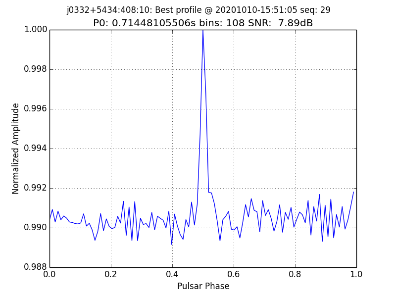
A recent observation from the CCERA site of J0332+5434 is shown below.

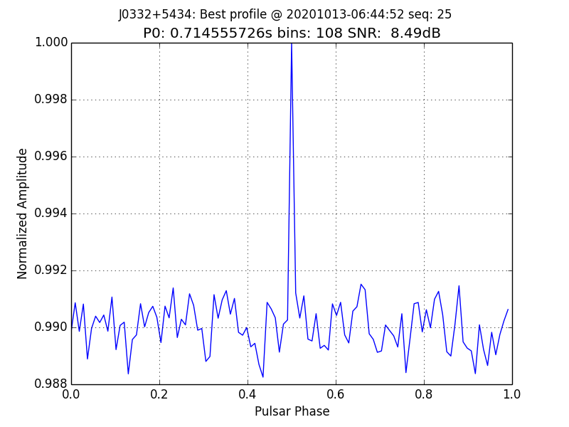
Real-time Display

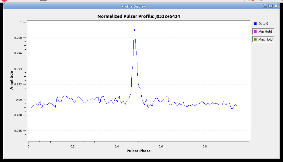
The main flow-graph includes an XMLRPC server, which means that external applications can query data objects with the flow-graph in real time.

One such application, profile_display, has been developed that is used to display the current accumulated pulsar profile. A screen-shot is show below.

Conclusions

Constructing a general-purpose Gnu Radio signal flow that provides both a filterbank (.fil) file and a collection of trial epoch-folded profile data appears to be perfectly feasible, even on modest compute platforms. The compute platform at ATA/HCRO is quite well-appointed, and that allowed experiments operating at sample rates as high as 25Msps without any sample drops or overruns. The Stupid_folder is implemented in Python and there was initial uncertainty about how well it would perform—but since it receives samples at what amount to “audio” rates, it is quite able to “keep up”. Explorations of millisecond pulsars may require revisiting the decision to write the folder in Python, but for general exploration of pulsars, particularly by small-scale institutions and amateurs, the current design appears to be more than adequate.