
Memo 0010: RFI excision techniques for riometry
Canadian Centre for Experimental Radio Astronomy http://www.ccera.ca
Memo: 0010 RFI excision techniques for riometry
To: Interested parties
Cc: Open Source Radio Telescopes
From: Marcus Leech, mleech@ripnet.com
Date: Feb 25, 2019
Subject: RFI excision in a modern riometer design
This memorandum describes a set of algorithms and techniques for the excision of RFI noise, in real-time, for an SDR-based riometer.
Riometers
A riometer is a special type of RF radiometer which measures ionospheric absorption using the galactic-background synthrotron emissions as a kind of “standard candle” against which absorption in the ionosphere can be measured. The term riometer is a coined term standing for Relative Ionospheric Opacity Meter. These instruments have been used for many decades to study the ionosphere and the effects of “space weather” on the ionosphere.
The riometer receivers typically operate in the range of 25 to 45MHz, usually in “windows of opportunity” somewhere in that spectrum. Conventional instrumentation usually consists of an analog measurement receiver using a Ryle-Vonberg “servo” to stabilize gain variations. In these instruments the “measured quantity” is the error voltage used to null-balance the Ryle-Vonberg control loop. Instrument detection bandwidths are typically between 10kHz and 250kHz.
The RFI problem
It will perhaps come as no surprise to the contemporary experimenter that the low-VHF portion of the spectrum has become a rich source of RFI and unwanted signals in the last two decades.
This situation leaves “conventional” riometers subject to extended periods where they provide data of very poor quality.
For example, here is a narrowband (about 250kHz) accumulated spectrum for a riometer operating near Ottawa, Canada:
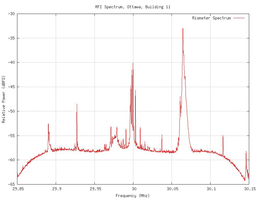
Example RFI spectrum captured near Ottawa
This type of spectral “pollution” is not uncommon in many current riometer deployments, and it is easy to see how a conventional “dumb” radiometer would have a very hard time producing long-term-meaningful data in such an environment. Statistical data showed that nearly all of the spectral features above are “transient”, but “persistent”. It is amusing to note that an annoying spectral feature that is non-transient in nature, and stable has very little negative impact on riometer measurements, other than perturbing the calibration of the instrument by adding a constant offset. It turns out that most RFI sources in this range are transient, however, and on time-scales that cause significant impacts to data quality.
Measurements
It should be noted that any RF radiometer, regardless of the presence of any techniques to stabilize its gain (Ryle-Vonberg servos, Dicke-switching, Reference-subtraction, etc) is simply measuring the area under the frequency-vs-amplitude curve. One can measure this area with a simple diode detector that is presented with some bandwidth-limited “chunk” of spectrum—it will faithfully produce a voltage output that is proportional to the notional area under this curve.
Most riometers operating world-wide today are “simple” radiometers using decades-old analog measurement techniques. The presence of gain-stabilizing techniques is due largely to the fact that decades-old RF devices had relatively “steep” gain-vs-temperature curves, and considerable device-to-device variability.
Spectral Measurements
The advent of digital signal processing technology and techniques means that new approaches to riometry in general, and the RFI-excision problem in particular, can be realised effectively and cheaply.
Recall that a conventional riometer conceptually measures the area under the amplitude/frequency curve, but it does so oblivious to the frequency-domain details of that curve. With modern, digital, techniques, one can measure the power spectrum over the selected bandwidth of interest with approximately as much ease as one used to measure the total power in a conventional instrument.
Once you have the power spectrum, computed with an FFT wth suitable parameters, you have a much better “view” into the activity within that spectrum. The ideal spectrum for any kind of instrument measuring natural noise phenomenon, like the galactic synchrotron background, would be quite flat. Indeed, it is this flat spectrum, and smooth changes in amplitude of that spectrum, that we are trying to measure—this is true in both ionospheric science and most radio astronomy as well.
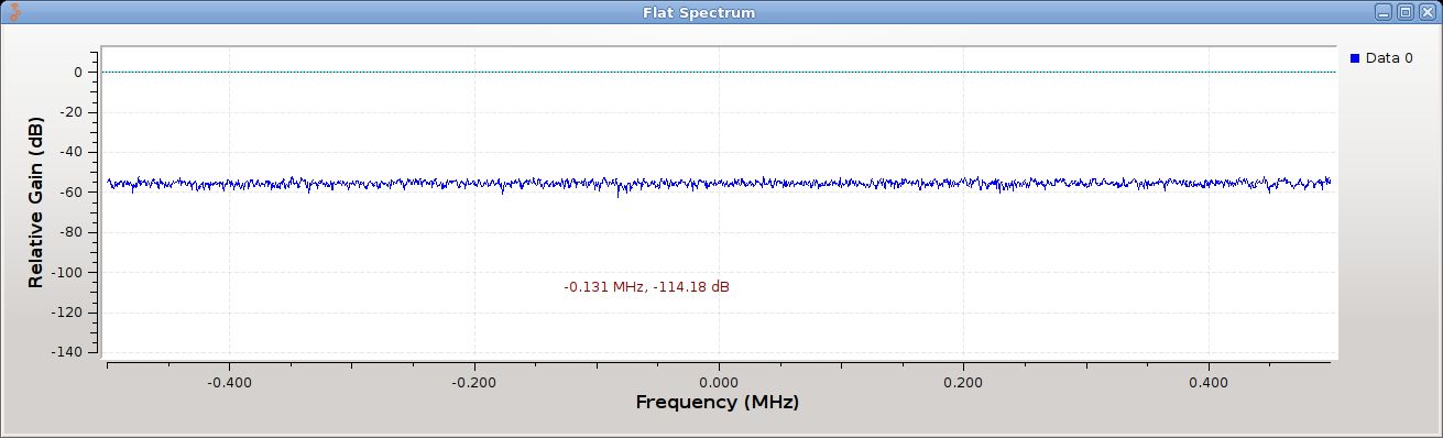
An idealized RFI spectrum, or “noise floor”
The RF engineer might refer to a such a “neutral” spectrum as the so-called “noise floor”. It represents the broad-band, “white” noise of both the instrument and whatever natural broad-band noise sources may be “visible” to the antenna.
Scientifically, we seek to measure the “noise floor” and smooth variations in the noise floor, consistent with instrument operational parameters. For a wide-beam riometer, we want to measure smooth changes in the noise-floor on timescales of a sidereal day. For a radio astronomy experiment, those measurements might evolve over timescales of minutes or seconds, as the object of interest transits the beam-pattern of the antenna.
When the spectrum is contaminated with Radio Frequency Interference (RFI), the spectrum, of course, does not have a “flat” appearance, and that means that the notional area-under-the-curve computations will be perturbed considerably.
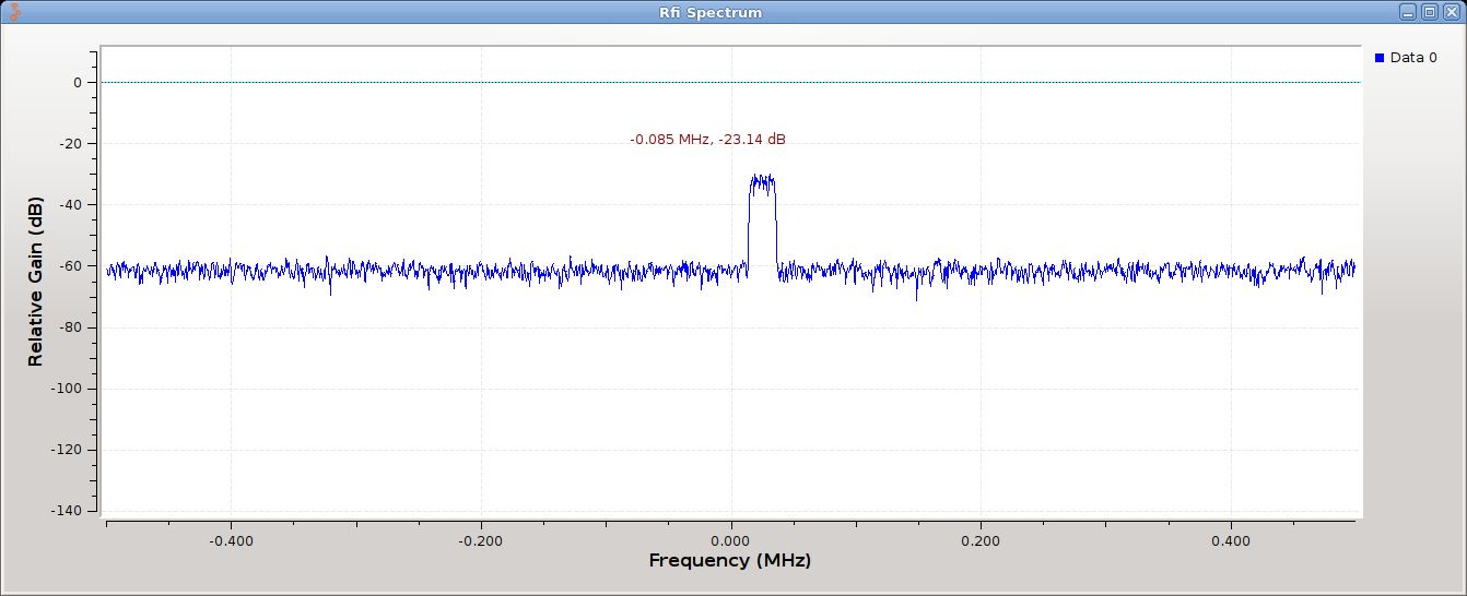
Simplified example of RFI intrusion
In the above, we can easily see an unwanted spectral visitor (in this case, simulated for clarity). It is a full 30dB (1000 times) “brighter” than the notional noise floor background. This will cause an unwanted, positive-going response in the detector. Since it occupies a small part of the total spectrum shown, that influence will be “diluted” by the ratio between its occupied bandwidth and the total bandwidth under observation by the detector (whether DSP or a diode).
In real RFI situations, of course, such “spectral visitors” are randomly distributed in the three time, frequency, and amplitude dimensions. They don’t always arrive as nicely isolated singletons, but often bring along friends, or join “parties in progress”. They’re a jolly bunch, to be sure.
Making the FFT work for us
When we start evaluating signals using the FFT, instead of a traditional “detector function” (whether that’s a diode in hardware, or a complex multiply in DSP), we can start to apply procedural heuristics to the data that results, in order to achieve desirable RFI outcomes.
An observation about a power spectrum that is sparsely contaminated with RFI is that most of the spectrum still represents the notional noise floor. If we define sparse to mean “occupies less than a meaningful majority of the FFT spectral estimate” then we can apply a simple algorithm to smooth the spectral estimate by:
- Compute the statistical mode of the FFT data set
- Compute the statistical minimum of the data set
- Combine the mode and minimum1 estimates using a weighting function into a new aggregate estimate
- Replace all members of the FFT data set that exceed the above estimate by some “reasonable” threshold with the above estimate. We use 2.2dB.
- Apply a small amount of statistical fuzz to the resulting data set.
Once you have computed a new smoothed spectral estimate, it is considerably more representative of the notional noise floor—and thus the scientific noise phenomenon we are trying to study.
The above algorithm procedure is necessarily heuristic in nature, and is not perfect. It can be overwhelmed in the presence of non-sparse RFI. It may be the case that a dynamic weighting function could be applied between the mode and minimum to produce better results in the presence of not-quite-sparse RFI spectral artifacts.
Impulse Noise
In the so-called “real world” (a place I have read about in the ancient texts, but have seen only thin evidence for otherwise), RFI shows up not only as discrete spectral artifacts, but also as broad-band, impulsive, noise.
Impulse noise tends to be spectrally “white” – it has the same amplitude across the spectrum of observation. This means that discrete spectral techniques as above will not be able to recognize it and excise it.
In order to recognize and ameliorate impulse noise, we must return to the time domain, since the frequency domain affords no special advantage.
Impulse noise tends to exist at multiple time-scales, and efforts to remove it must consider the time-scales of impulsive noise that are detrimental, and those that are scientifically interesting. In riometry, for example, various types of solar radio noise bursts are scientifically interesting, and automatic excision may not always be an ideal approach.
But many types of artificial impulse noise operate over time-scales where relatively simple time domain filtering techniques can be used without detrimental effects on the scientific data quality.
In our case, we use a length=9 median filter to remove impulse noise over the smaller timescales that are typical of artificial impulse noise. The excised FFT is treated as a vector of power estimates (which it is), and each element of the vector has a median filter applied to it. The median filter has the side-effect of decimating the data stream, since it considers 9 samples at a time, and returns only a single estimate.
The median filter accumulates 9 samples, where each “sample” is an FFT-sized vector. It then sorts those vectors of samples, and discards all but the 3 inner (mid value) samples, and returns their average. This has the effect of discarding the “statistical outliers” and is reasonably effective at removing impulse noise operating at time-scales of approximately 20-100msec.
For impulse noise of larger temporal scale, a second layer of moving-median filter is employed with longer lengths, and slower sampling rate. This is implemented in the detector power (single-value) domain, instead of the frequency domain. This second layer uses an L=17 moving median filter, which can remove impulse noise on timescales up to roughly 2 seconds.
It is important to realize that increasing the time-scales over which median filters operate creates a “science hazard” in which events such as Solar radio bursts, and short-time-scale absorption events operate — a more aggressive median filter scheme will tend to suppress these events partially or completely.
Pulse Gating
It is sometimes the case that very-large broad-band impulses are seen that cannot be excised using any of the above techniques. In those cases, we simply “gate” the input whenever there is a sudden increase in input power that exceeds a healthy threshold. Once this happens, the input is gated until the input returns to its previous level. This is very similar to the noise blankers that are quite common on HF communications receivers. The threshold is chosen so that events like solar noise bursts are unlikely to trigger it.
Post-facto vs Real-time
The techniques described here can be applied either in real-time, or in a post-facto data-cleaning procedure. A significant down-side to the post-facto approach is that it requires that spectral data be recorded at a high enough rate to allow these algorithms to work correctly. That leads to a much larger storage requirement, in exchange for a much-smaller real-time CPU performance requirement. It can be observed that these algorithms have been tested to work on relatively modest ARM-based single-board computer systems, albeit at slightly-reduced update rates (30Hz vs 50Hz).
Conclusions
We describe what is very much a “work in progress”. The nature of these types of algorithms is that they require modification as they are exposed to different types of environments. Testing in real-world conditions has indicated “promise”, but much more experience is still required.
It should also be noted that the literature is well-populated with descriptions of RFI-excision techniques in radio astronomy, and that we make no claim as to originality. Other experimentalists in this domain have applied similar techniques.2
1 For a non-tilted spectrum the mode and minimum will be numerically close
2 See the work of Glen Langston on median filtering in radio astronomy, for example:
https://github.com/glangsto/gr-nsf