
Ken Tapping
National Research Council
Marcus Leech
Science Radio Laboratories, Inc.
Abstract
We describe alternatives to Dicke radiometers and phase-switched interferometers for small-scale radio astronomy. Instead of moderately-complex, hardware-based switching hardware that is often difficult to obtain or expensive, these designs use cheap, widely-available software-defined radio RTLSDR 1 “dongles” and free Gnu Radio 2 and simple_ra software.
1. Background
Radio astronomy almost always involves measuring a very small part of the output from the radio telescope receiving system that is added to a much larger contribution due to receiver noise and emissions from the ground and sky. In principle the desired signal can be extracted by “backing off” the signal voltage due to the other contributions. However, in practice this often does not work well because the gain of the receiving system inevitably drifts with time. If the desired signal is in the region of 1% of the other output contributions, which is fairly typical, a drift of 1% in the system gain acting on the background noise alone will make the output drift by an amount comparable to the output change due to the cosmic source. This will make it hard or even impossible to identify the source. This problem has been around since the beginnings of radio astronomy so solutions have been around for decades. For single-antenna radio astronomy the Dicke system was developed (named after its inventor, Robert Dicke) and for interferometers, the phase-switched interferometer is widely used.
These systems date back the the 1950’s or earlier, and technology has improved dramatically since then. Receivers are far more sensitive, developing very low levels of internal noise, and are much more stable. Gain drift on modern receivers is far smaller, and those drifts operate on far lower noise levels. Today we can do most of the signal processing in a digital environment, which is also much more stable than the equivalent analogue signal processing systems. In addition, the hardware today is much less expensive, which allows us to adopt measures that would have been impractical even a few years ago.
In backyard and small-instrument radio astronomy, the most common instrument configurations for continuum astronomy or low-sensitivity solar observations are the Dicke radiometer and the phase switched interferometer. We have developed SDR-based alternatives to both of these systems.
2. The Dicke Radiometer
2.1 The Standard Implementation
A single antenna radio telescope, pointing at a region in the sky where there is a radio source would produce an output voltage (assuming square-law demodulation):
V out = Γ(T sys + T Ground + T Sky + T Source) =Γ(T∗+T Source)
In the equation Γ incorporates the gain-bandwidth product of the receiver, Boltzmann’s constant (the conversion factor between temperature and energy), and the relationship between input power and demodulated voltage. We can lump all the unwanted contributions together into one value, T. If T is 300K and T Source is 1K, a change in Γ of 1% will change the receiver output by 3K, which is larger than the source signal. It will be nearly impossible to identify the source.
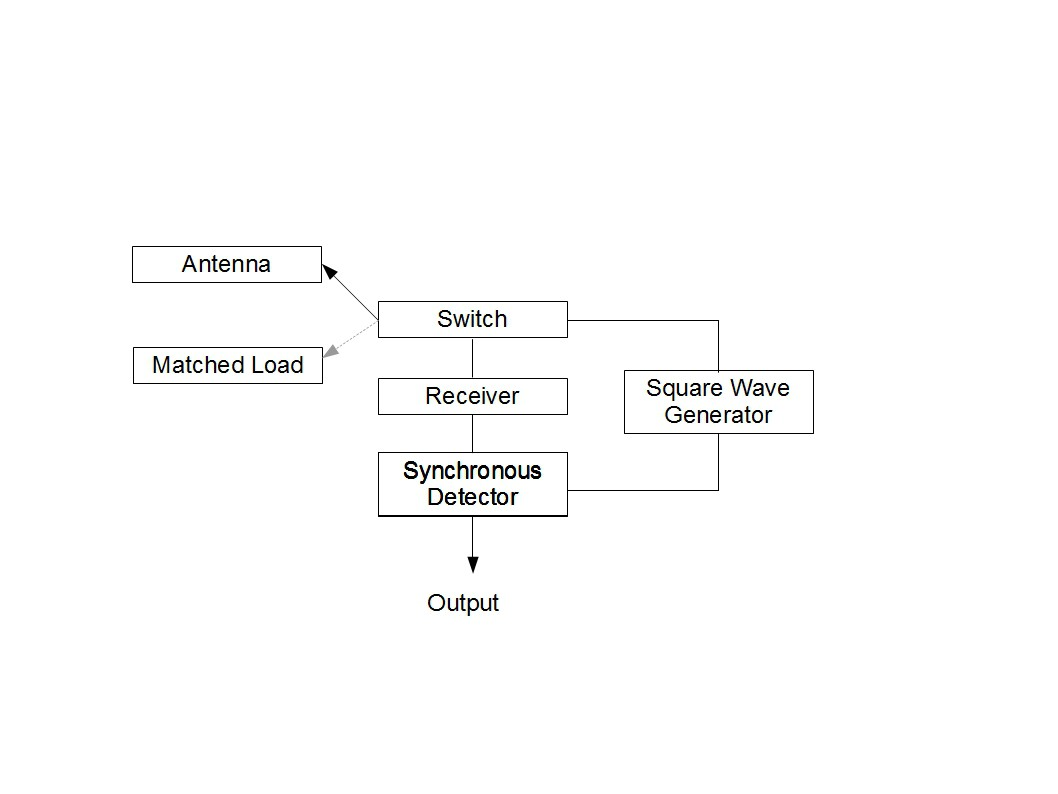
Schematic of main components of a Dicke radiometer
The figure above shows the main elements of a Dicke radiometer. A switch at the receiver input is toggled between the antenna and a matched load at a rate faster than Γ can reasonably vary, typically hundreds of times a second. The operation is controlled by a master square wave generator. The output from the receiver passes to a synchronous detector which, driven by the square wave generator, inverts the signal when the load is connected and does not invert it when the antenna is connected. The output from the synchronous detector passes to a low-pass filter or integrating circuit that adds the non-inverted antenna signal to the inverted load signal, which is equivalent to subtracting them. When the antenna is connected the receiver output is
V (antenna) = Γ( T sys + T Ground + T Sky + T Source)
When the load is connected the output is
V(load) =Γ( T sys +T Load)
Subtracting the load equation from the antenna equation gives simply
ΔV =V (antenna)−V (load) =Γ( T Source + T Ground + T Sky −T Load)
If the system noise temperature is the main contribution to the unwanted part of the receiver output this procedure will give a significant improvement in output stability and the ability to see the receiver output changes due to the source being observed.
At centimeter wavelengths this might not be sufficient. Sky noise is significant and changes rapidly over time-scales of seconds. Thermal noise from the ground is also picked up by the antenna, which changes with time and antenna position. This led to a modification to the Dicke radiometer known as beam-switching. At centimeter wavelengths the antenna is usually a dish, and in the beam-switching radiometer the load is replaced by an auxiliary feed horn, located close to the signal horn. This horn sees almost the same bit of ground and the same area of sky as the signal horn, but does not see the source, so when the receiver is connected to the signal and reference horn the output equations are respectively.
V(antenna) = Γ( T sys + T Ground + T Sky + T Source)
and
V(reference) =Γ( T sys + T Ground + T Sky)
So subtracting the two equations gives
Δ V =V(antenna)−V(reference)=Γ T Source
This makes beam-switching a very powerful technique.
2.2 The RTLSDR+Gnu Radio Version
The standard implementation of the Dicke radiometer dates back to a time when receivers were significantly more noisy, and much less stable than their modern cousins. In addition, components are now considerably less expensive. This allows a relaxation in some of the rigour of the original configuration:
- One can make two identical receivers with their respective components located close together, on common heat-sinks, in the same insulated container, power them from a common power supply and assume both will reflect the same gain-bandwidth drifts with temperature, power supply variation etc. This is made easier by the components being significantly smaller.
- One can digitize the signals before demodulation, which removes a lot of analogue signal processing and provides a better and more consistent demodulation process.
- The key receiver back-end and demodulation components are available in cheap, small devices (RTLSDR dongles and other SDR devices such as USRPs).
- The software is available already.
This makes possible a modern revision of the Dicke Receiver…
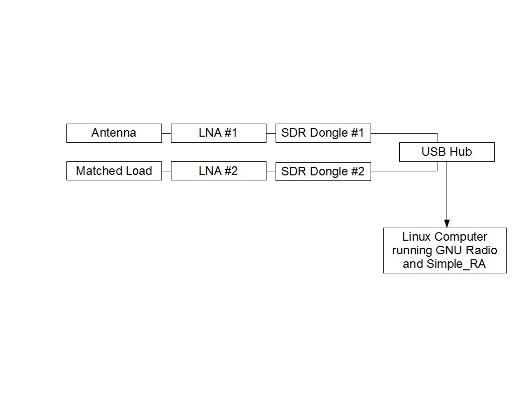
A modern revision of the Dicke Receiver
Two identical low-noise amplifiers are attached to a common heat-sink in a common container. One has its input connected to the antenna and the other to a matched load that is either attached to the heat-sink or to some other thermal mass. The two RTLSDR (dongle) receivers are attached directly to the LNA outputs. The dongles provide additional amplification and filtering, along with base-band down-conversion and sampling. The rest of the dongle electronics, specific to the purpose the dongles as intended (FM radio, DVB-T TV, etc) are bypassed, yielding a stream of in-phase and quadrature (I/Q or complex baseband) samples that are processed by the computer. The hub merely provides a means to collect the signals into one cable if the dongles are a long way from the host computer, otherwise the hub can be left out.
The outputs of Dongle#1 and 2 are respectively:
V(antenna) =Γ1( T sys + T Ground + T Sky + T Source)
and
V(load) =Γ 2 (T sys + T Load)
If the components are identical and the points in the list are followed, then after initially putting in an attenuator into one of the receivers to balance the noise levels, we can then assume that
Γ 1 =Γ 2 =Γ
and the same subtraction can be made as in the case of the standard Dicke radiometer:
Δ V =V(antenna) −V(Load) =Γ(T Source + T Ground + T Sky −T Load)
except now there is no switching process. If an auxiliary feed is attached to the dish antenna, and the load channel is connected to this, an SDR-based version of the beam-switching process occurs, yielding the same result:
Δ V =V ( antenna)−V ( ref.beam)=Γ T Source
We show below, a fragment of a Gnu Radio flow-graph that demonstrates the simple data-flow required to produce a differential radiometer response, given the above-described hardware configuration.
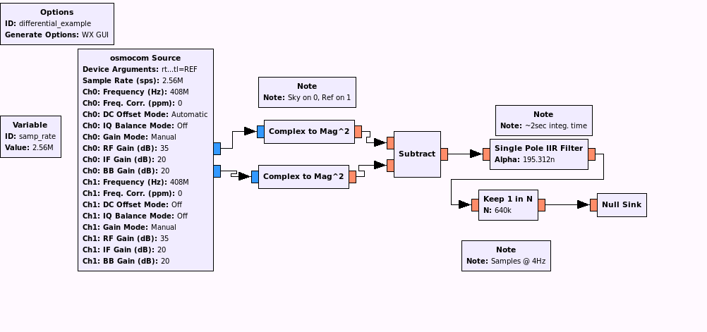
A Gnu Radio flow-graph demonstrating the simple data-flow required to produce a differential radiometer response.
In the so-called flow-graph shown above, the two complex base-band data streams are delivered to a block that acts like a conventional detector, computing:
P est =I^2 + Q^2
These two blocks each produce the instantaneous power estimate for both the sky and reference channels. The reference estimate is subtracted from the sky estimate, and then filtered (integrated) with a single-pole IIR filter and decimated down to a lower sample rate of 4Hz. Ordinarily, such a flow- graph would include data-recording and display functions, we show here only the “heart of the matter”.
The plot below is a transit of the Milky Way observed at 408 MHz using a 10ft dish and a dual RTLSDR dongle differential receiver as described here. The vertical ordinate is the difference between the outputs of the antenna and load channels, so it can be positive or negative. This transit is part of the data being accumulated as part of a sky survey.
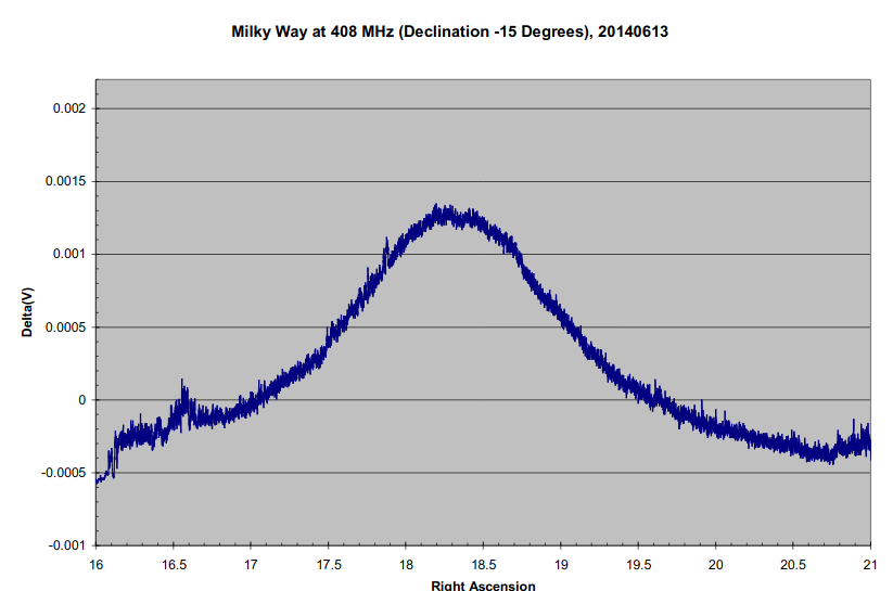
Plot of a transit of the Milky Way observed at 408 MHz using a 10ft dish and a dual RTLSDR dongle differential receiver.
Below, we show the plot of a daily solar transit, recorded at both 10.7cm and 2.6cm wavelengths, where the 10.7cm data are derived from a fixed-load differential radiometer, and the 2.6cm, from a reference-beam differential radiometer, as described previously.
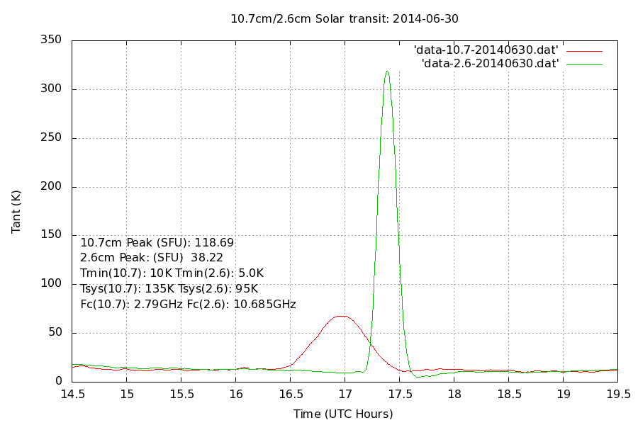
A daily solar transit recorded at both 10.7cm and 2.6cm wavelengths.
The software is a Gnu Radio based application, simple_ra, which runs under Linux and can be downloaded from the CGRAN 3 website.
3. The Phase-Switched Interferometer
3.1 The Standard Implementation
It is best to start this discussion with the basic (adding) interferometer. This consists of two antennas in an east-west line, separated by many wavelengths.Two antennas, separated by a distance D are observing a source at an angle β from the meridian.
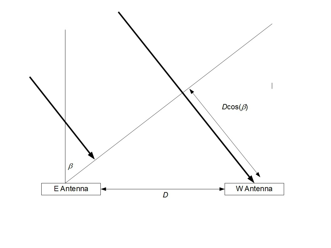
Two antennas separated east-west distance simultaneously observing a source east of the meridian. The signal reaching the west antenna travels an additional distance undergoes a phase shift.
The signal reaching the west antenna has an additional distance of Dcos( β ) to travel. This corresponds to a phase difference of:
Δφ = (2pi D)/λ cos β
where λ is the observing wavelength. The normalized signal power received from the source would then be
T(β)=T 0 G(β)(1+cos Δφ)
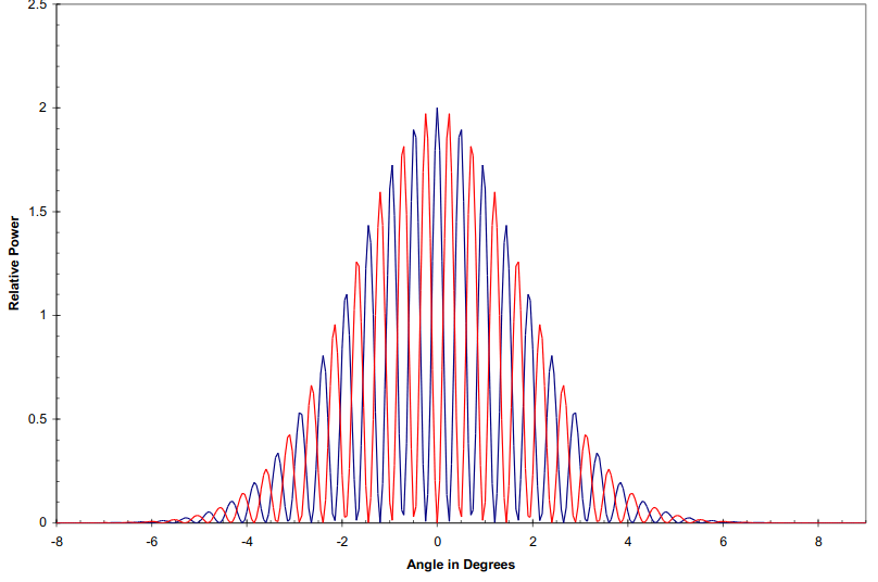
where G( β ) is the gain of one of the two (identical) antennas. T 0 is the signal from the source when observed on the meridian. For example, two 3-m antennas 50 metres apart, connected as an interferometer operating at a wavelength of 21cm would produce an idealized response approximately as shown in the figure below.
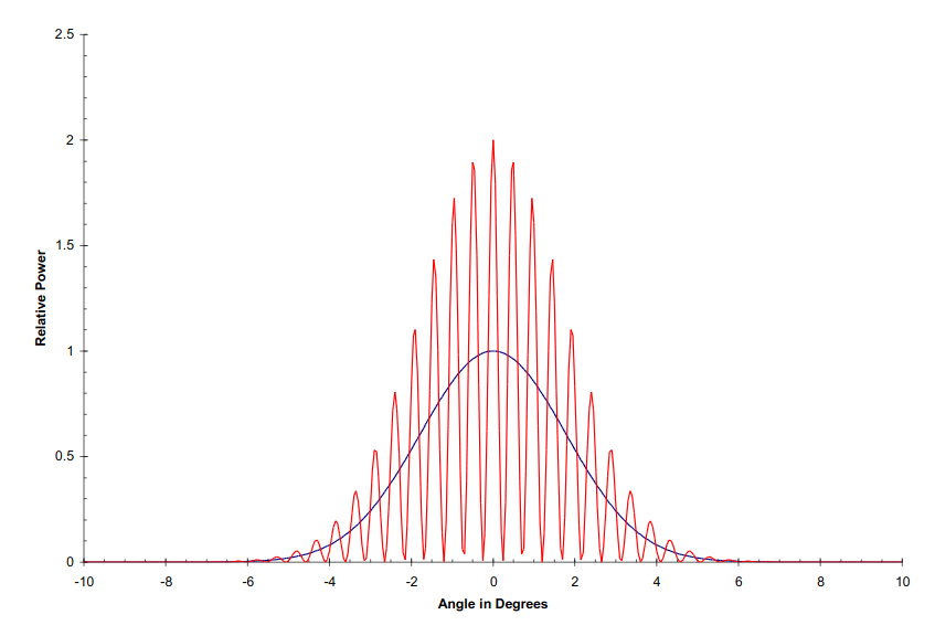
Idealized response for two 3-m antennas operating at a wavelength of 21cm 50 metres apart.
The black line shows the sensitivity pattern of the individual antennas; the red line shows the interference pattern due to the interferometer. The hardware arrangement is shown below.The hardware arrangement includes Low noise amplifiers at the antennas to compensate for the cable losses.
The hardware arrangement is shown includes low-noise amplifiers at the antennas to compensate for cable losses.
Low noise amplifiers are included at the antennas because of the losses due to the long cable lengths running along the interferometer baseline. We assume here the lengths are equal, although they don’t really have to be.
However, the situation depicted in the figure is is not the whole story. Not shown in the plot are the noise contributions from the receiver, ground and sky, so the receiver output is more accurately given by
V 1 =Γ(T sys + T Ground + T Sky +T(β(φ)))
It is useful to observe that if we add a phase shift of 180 degrees to the phase difference Δφ , all the maxima in the fringe pattern turn to minima, and vice versa.
V 2 =Γ(Tsys + T Ground + T Sky +T(β(φ + pi)))
The non-shifted and shifted antenna patterns are shown, idealized, in the next figure.
Idealized non-shifted and shifted antenna patterns.
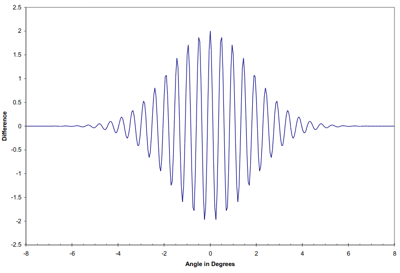
So if we switch a 180 degrees phase shift in and out at a rate faster than the gain variations and then synchronously demodulate the receiver output in the same manner as in the case of the Dicke radiometer, we get
ΔV =V 1 −V 2 =Γ(T(β(φ))−T(β(φ+pi)))
An idealized response at the output is shown in the next figure.
The hardware for a conventional, phase switched interferometer is shown below.
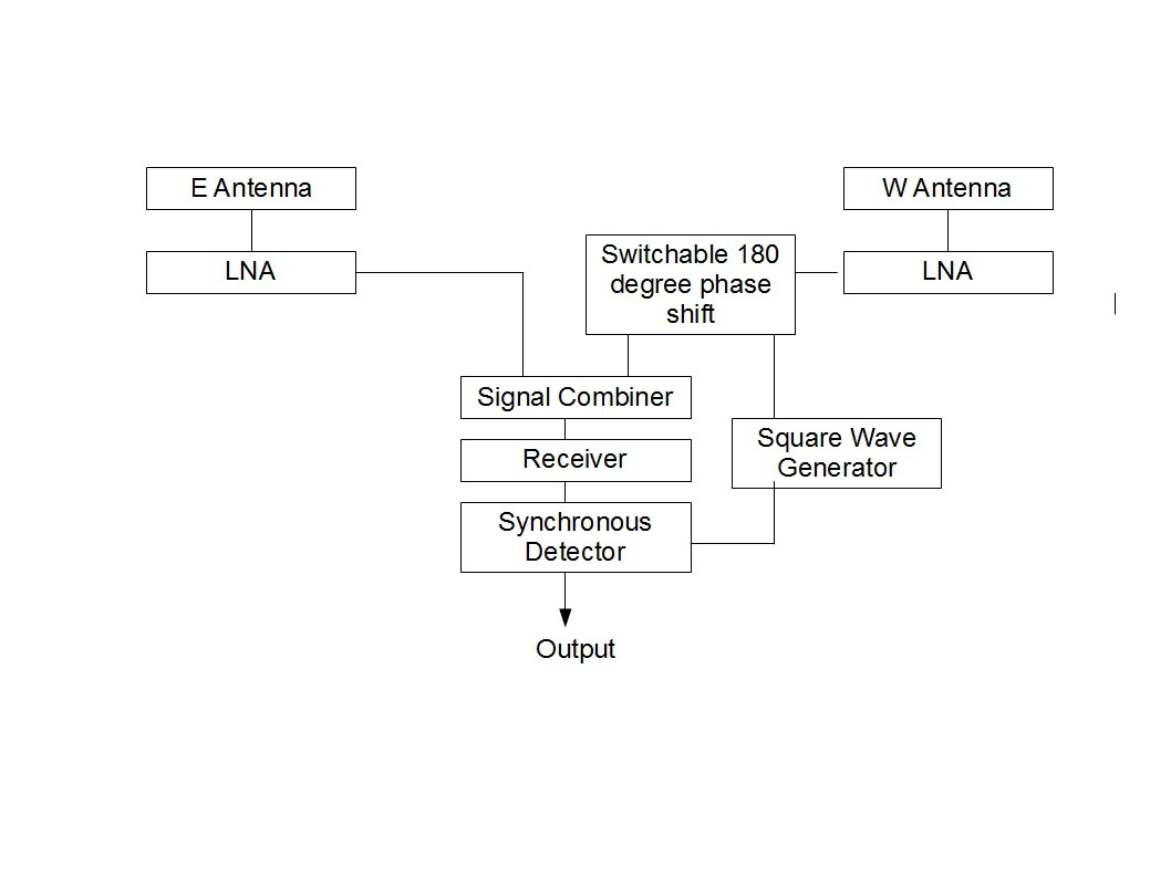
Hardware for a conventional, phase switched interferometer.
3.2 The RTLSDR+Gnu Radio Version
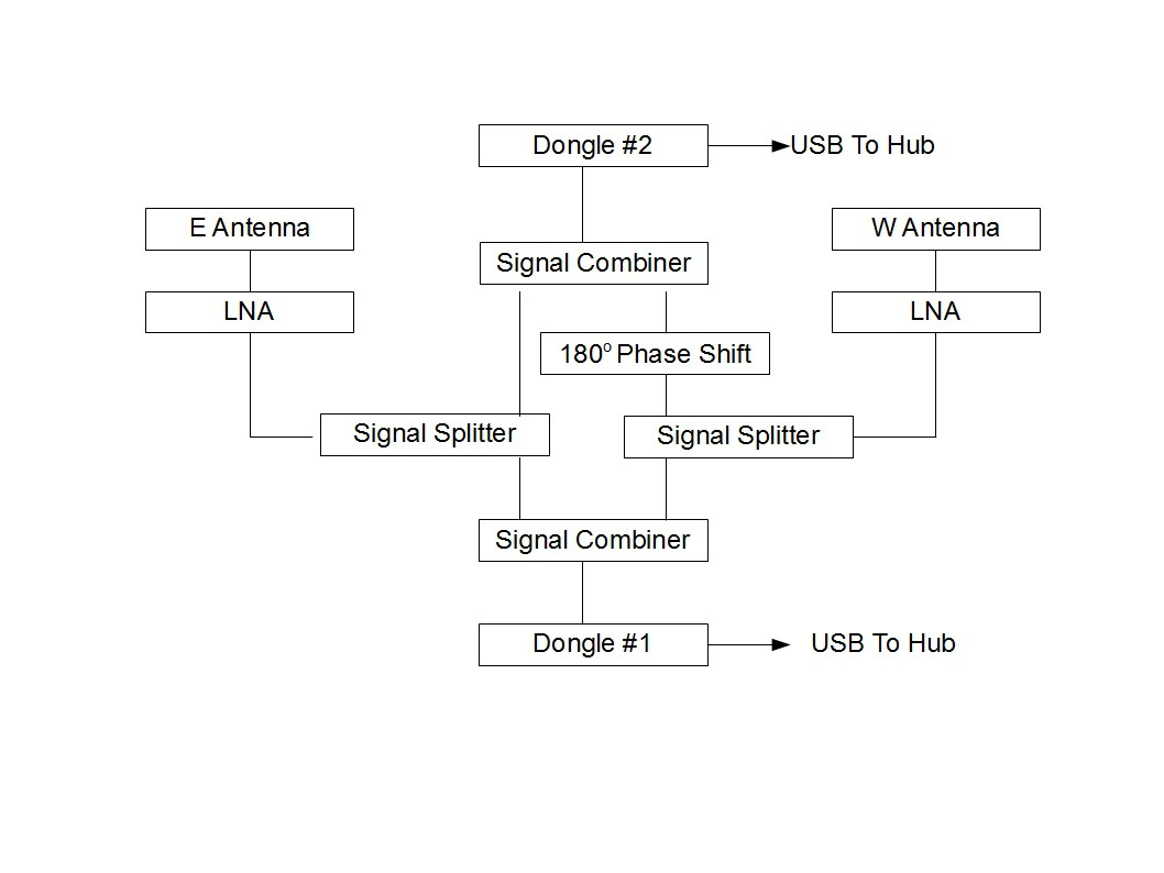
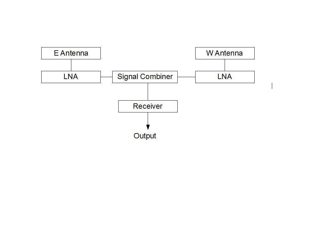
RTLSDR dongle+Gnu Radio based equivalent of a phase-switched interferometer.
The diagram shows the arrangement of a RTLSDR dongle+Gnu Radio based equivalent of a phase-switched interferometer. In the diagram, signal combiners and splitters are the same devices. They can be used to split a signal into two in-phase outputs or to add two signals to a common output. The signals from each antenna/LNA are split. One path from each antenna are simply added in-phase, and the other antenna has one path phase-shifted by 180 degrees. In this way Dongle #1 records the normal fringe pattern and Dongle #2 records the fringe pattern with the maxima and minima reversed. These are then subtracted. This is exactly equivalent to the signal processing in a normal phase-switched interferometer but with the processing being essentially continuous, occurring at the sample-rate of the incoming samples.
A proof-of-concept system has been assembled for operation at 137 MHz. The antennas used for the test were a dipole and reflector for the east antenna and a 14-element yagi for the west antenna. No cosmic sources have been observed with it yet, but the operating principle has been tested using satellite signals. Two examples are shown below. Since the satellites cross the interference pattern on oblique paths, the traces are complex, and as they do it rather quickly, the fringes are somewhat under-sampled, since the satellite fringe-spacing is on the order of six seconds, and the data are logged at a rate of once every two seconds.
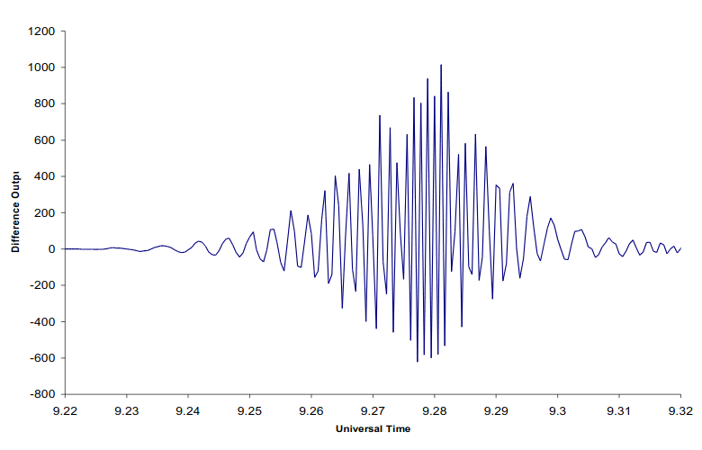
A proof-of-concept system operating at 137 MHz has been tested using satellite signals.
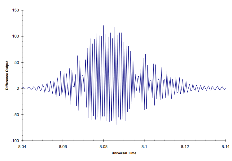
In both cases the transits show some asymmetry, probably due to a combination of the phase shift not being exactly 180 degrees (a half-wavelength piece of coax was used) and also the gain of both LNA+receiver channels probably differ slightly.
- See: http://sdr.osmocom.org/trac/wiki/rtl-sdr
- See: http://www.gnuradio.org
- Http://www.cgran.org3.