
Memo 0011: A 21cm map of the northern sky
Canadian Centre for Experimental Radio Astronomy http://www.ccera.ca
Memo: 0011 A 21cm map of the northern sky
To: Interested parties
Cc: Open Source Radio Telescopes
From: Marcus Leech, patchvonbraun@gmail.com
Date: Nov 1, 2019
Subject: A 21cm map of the northern sky
This memorandum describes the equipment and techniques used to produce a good-quality brightness map of the northern sky at 21cm wavelength.
Sky Maps
There are a plethora of observing regimes and projects that are routinely used in radio astronomy, but the production of a sky map is a project that is easily accessible to the amateur observer, and produces satisfying results.
Such a map shows the brightness distribution over the sky for a given set of observing wavelengths. In the case of the 21cm hydrogen line wavelength, maps show the distribution of hydrogen over the sky. For amateur observers, such maps generally show the distribution within our own galaxy, since extra-galactic hydrogen is considerably more faint, and significantly red/blue shifted relative to the rest frequency of 1420.40575MHz, due to relative motion between the observer and the target extra-galactic hydrogen.
21cm emissions in the interstellar medium
Hydrogen is the most abundant element in the universe. Neutral hydrogen atoms occupy the space between the stars, in vast clouds throughout our galaxy. The density of these atoms is quite low—a few dozen atoms per m3 of the interstellar medium. But when considered in bulk, the columnar brightness is considerable, and easily observed by modest equipment.
The emission mechanism is due to the hyper-fine splitting of the ground state of neutral hydrogen, where a collision occasionally causes a spin-flip, with the emission of a photon with a frequency near 1420.40575MHz, or a wavelength of 21.11cm. For any given atom, the transition probabilities are low, yielding rates between 1.0e-5 and 1.0e-6 years. But along any given line of sight, there are an unfathomable number of atoms undergoing this ground-state transition at any given time—yielding a relatively bright astronomical “signal”.
Doppler Shift
Nothing is ever really “standing still” in this universe, and that is certainly true of clouds of hydrogen relative to observers here on earth. The magnitude of the peak relative motion of galactic hydrogen is roughly +/- 200km/sec. This corresponds to a frequency span of approximately +/- 1MHz from the notional center frequency of 1420.40575MHz.
The line also tends to be “spread” due to the statistical velocity distribution along any line of sight—the notional Doppler velocity is a “central tendency” with a Gaussian-like distribution around the notional velocity. This spread is typically on the order of 20-30 km/sec, or approximately 100kHz.
Radio Telescope
The radio telescope used to produce our 21cm sky map starts with a spun-aluminum 1.8m dish, located on the roof of our facility, near Smiths Falls, Ontario, Canada. The roof is at a level approximately 8.5m above ground, which reduces the ground clutter, and improves our horizon pointing.
The dish is fed with a circular wave-guide feed, constructed from 15cm (6”) HVAC duct, with a small brass probe on a type-N connector attached to the side of the waveguide.
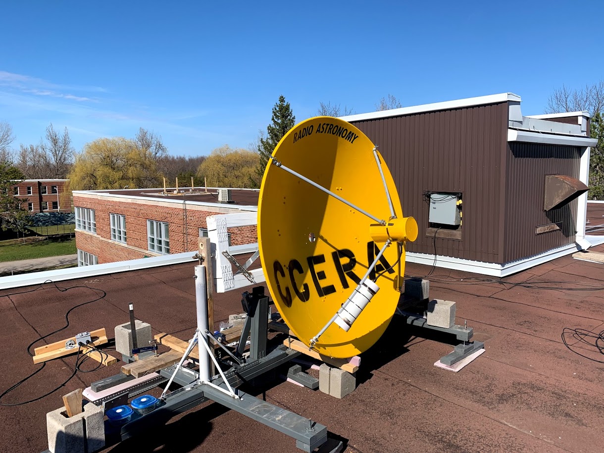
The 21cm dish.
The feed is connected to an off-the shelf Low Noise Amplifier (LNA) assembly, providing approximately 40dB of sub-0.7dB NF gain. The LNA was provided by NooElec1 as a prototype unit which is now available as a production item.
This LNA drives approximately 50m of RG6 coaxial cable, where it enters our laboratory through a bulkhead panel and is then amplified again with a 15dB line amplifier. The signal is then filtered with a dielectric filter and then split and fed to two Airspy R22 SDR receivers. The receivers acquire their master clock from and external GPSDO made by Ettus Research3. When locked to GPS, this gives a residual frequency uncertainty of approximately 1PPB (1 part in 1.0e9), or a velocity uncertainty of 0.0002 meters/second at 200km/sec notional Doppler velocity.
Each receiver is connected to an Odroid XU4 single-board ARM computer, running our odroid_ra software.4 An X86 host PC collects the spectral information over a 1Gigabit Ethernet network from the two Odroids and produces a file record every 30 seconds, giving a spectral estimate (in dB), and related housekeeping information (UTC time, LMST, frequency, bandwidth, declination, etc). Having two receivers on a single antenna feed gives us experimental flexibility, but also allows for slightly improved SNR with two independent estimates of the same signal.
The spectral files produced are somewhat voluminous, at approximately 75Mbyte/day. This could be reduced considerably by reducing the FFT resolution (currently 8192 bins) and logging estimates less frequently—perhaps once every two minutes. But the extra flexibility and spectral/temporal resolution allows for more detailed future data-processing exercises.
Motion control
The dish is arranged to operate in the so-called “transit” mode, in which the azimuth axis is fixed to point along the local meridian line, and the elevation axis is free to move. In our case, the elevation axis is driven with a simple linear-actuator or “motorized jack-screw”, with motion feedback from a USB-based elevation sensor from Level Developments5.
An inexpensive ARM-based SBC is attached to the back of the elevation yoke, and controls elevation via a relay module configured as an H-bridge. It is commanded remotely via a WiFi network connection from a WiFi router on another section of the roof.
A so-called motion scheduler moves the dish by 5 degrees elevation every 25 hours, ultimately covered a declination range from -35 in the South to +70 in the North.
Post processing6
Spectral estimates arriving from the two receivers are averaged together before being logged. The resulting data is still in a “raw” form, as shown below in a plot.
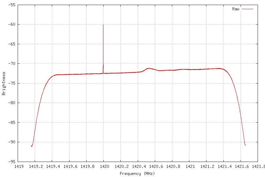
Raw data plot
It is immediately obvious that there are some artifacts that must be dealt with in order to proceed with further processing. This processing is performed using the “makepixels.py” tool in the maptools package. The edges of the plot fall-off steeply, which is to be expected with any band-limited signal, so our first job is to reduce the “view” to eliminate the “edge roll-off”:
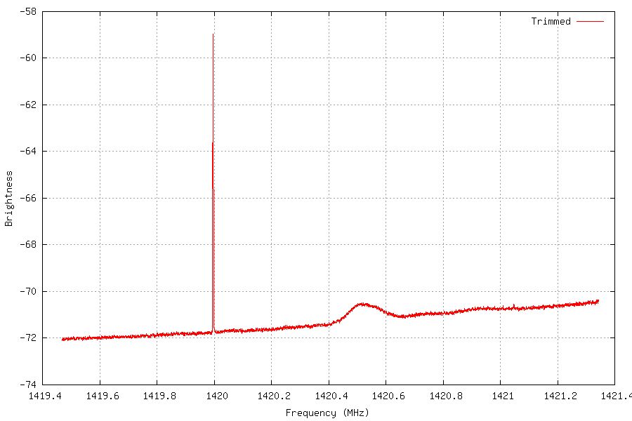
Drop-off eliminated
This has nicely eliminated the “edge roll-off”, but we still have a narrow-band artifact (in this case, from the receiver itself) at exactly 1420 MHz (the 142nd harmonic of the 10MHz reference clock). It’s also important to note that there’s an obvious “passband slope” in this plot, which is, again, an instrumentation artifact.
We can easily remove the slope by estimating it automatically and applying a linear correction— in this plot, the values have been converted into linear measurements, from the dB in the previous plots:
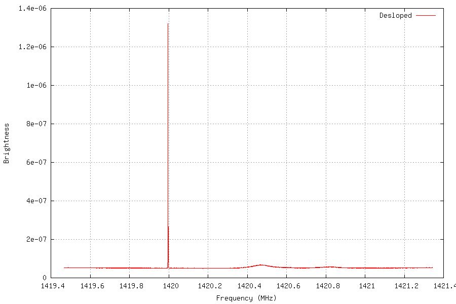
The slope – an instrumentation artifact – corrected, and the logarithmic data now linearized.
Next the data are converted into a temperature profile, given some calibration constants based on receiver characteristics, and large excursions above the minimum are removed (removing the spike at 1420MHz, or at least reducing it to inconsequential levels).
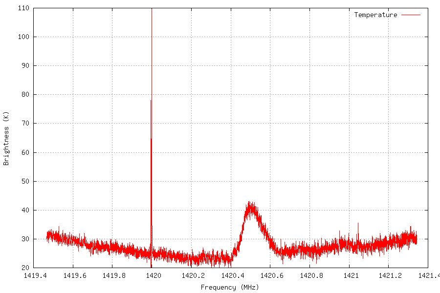
Brightness now calibrated as temperature
Here we can see the data have been converted to Kelvin, and the spike at 1420 is quite a bit smaller than it otherwise would have been.
The result is nearly ready to estimate the total brightness temperature, but there’s now a “dish” curve to the baseline that is a processing artifact that can be compensated somewhat:
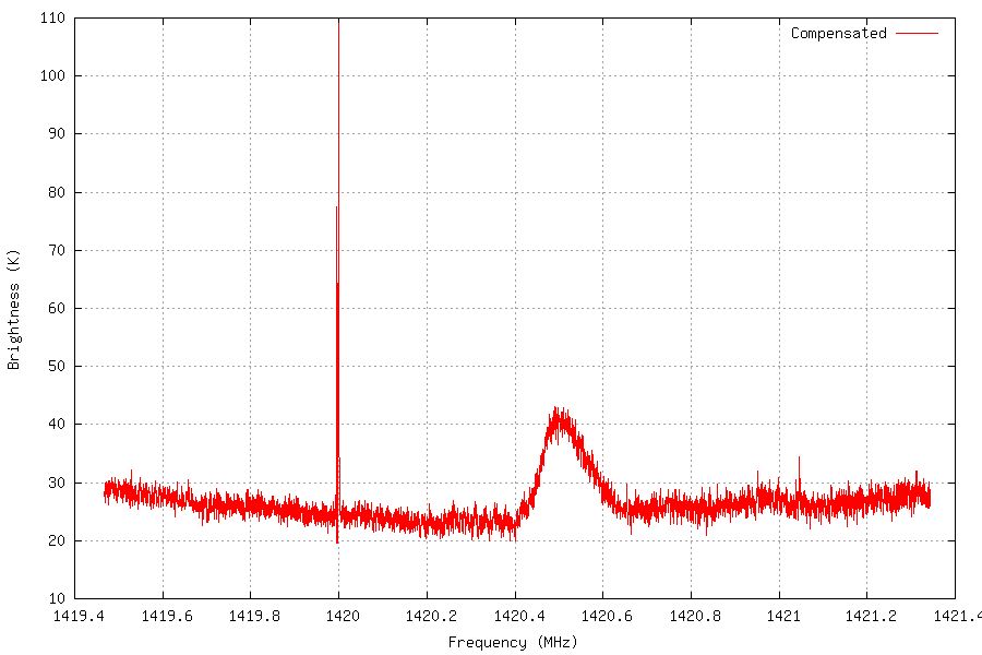
Final compensated data
From this corrected profile, we can calculate the total brightness temperature over the given frequency range (corresponding to a Doppler velocity range of approximately -160 to +160km/sec). This is simply a matter of summing all the bins, producing “pixel” of brightness estimate which is used to update a long-term averaging array. The code produces “pixels” that are approximately 5deg x 5deg, which corresponds to approximately ½ of the beam-width of the instrument. Each such “pixel” is stored as a single floating-point number in a file that is labeled with respect to its equatorial coordinates (recall that the spectral data records include this information).
It is important to note that in the processing of the raw spectral data, the temperature estimates are effectively “baselined” which removes some continuum information, but also eliminates, or significantly reduces, the effects of gain variation. It is a particular characteristic of spectral data such as that from neutral hydrogen that allows one to ignore continuum effects on the baseline and still produce meaningful sky temperature estimates.
Making images: the final map production
The goal of an amateur sky-mapping exercise is to provide an immediately-meaningful visualization of the accumulated data.
Recall that each “pixel” of total brightness data is stored in a file. The map-making procedure (“pixels.py”) uses these files to build a visual image of the data in a X/Y “heat–map”.
The procedure is fairly straightforward—the data are placed into a 2D array that is twice as large in declination is expected from the pixel files, with the intermediate rows being synthesized from the two surrounding rows of declination using straightforward 2-point averaging.
The 2D array data are then passed to routines in the matplotlib python library which is then saved as a PNG image:
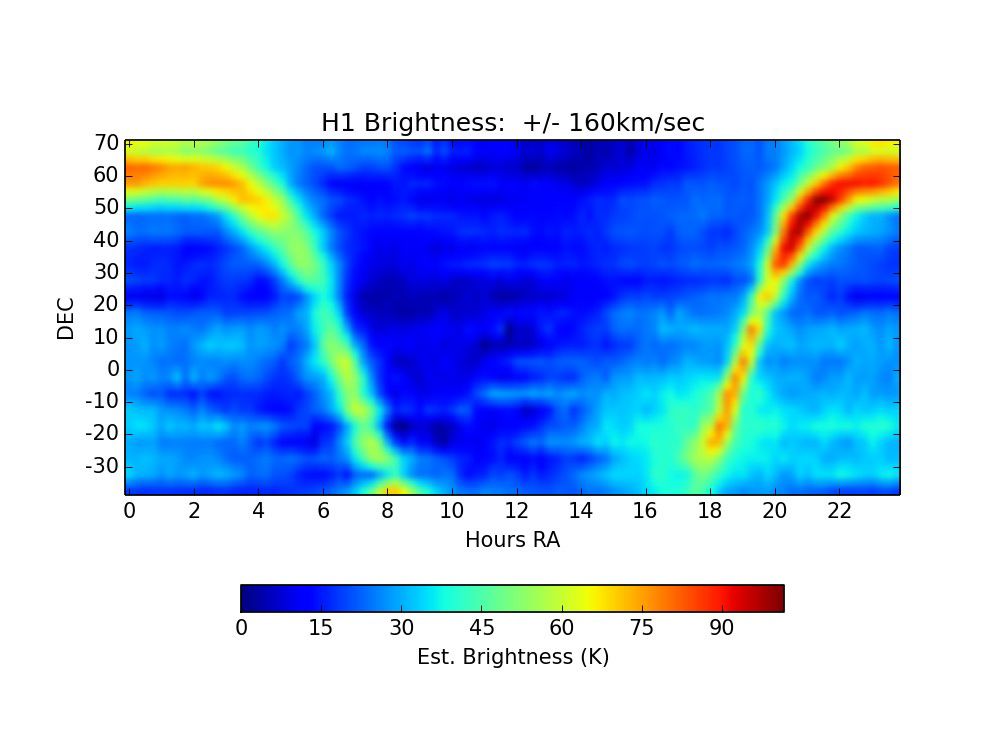
The temperature data colour-mapped in declination and right ascension. The disk and nuclear region of the Milky Way are apparent
The heat-map image can be improved in terms of visual appeal and contrast by processing with Gimp (an open-source tool similar to Adobe Photoshop).
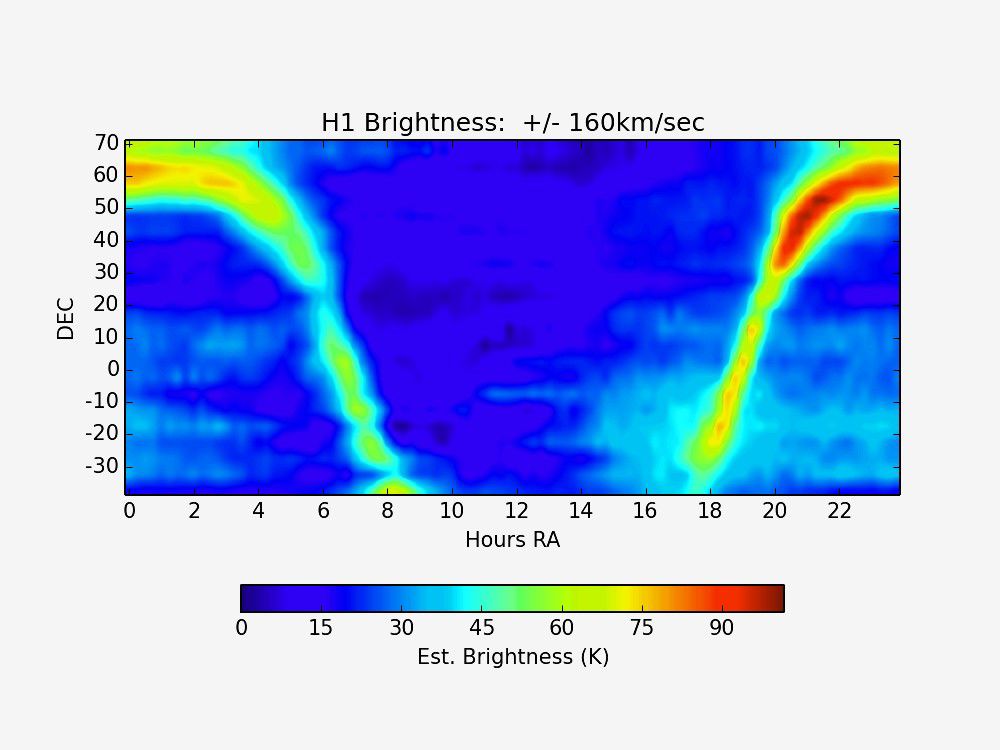
Prettified map
Conclusions and Further Work
An amateur-scale, modestly-budgeted instrument is easily capable of producing a complete sky-map covering a significant fraction of the sky available to the observatory. Modern Python libraries, such as Matplotlib, make the task of producing a visual heat-map quite straightforward.
Tools such as Gimp can be used to improve the visual appeal of such heat-maps, and to elucidate deeper details in a simple heat-map image.
Future work on the map-making tooling will extract sub-banded data from the input spectra, and produce a map that provides both sky temperature and red shift information in a single image.
- See: https://www.nooelec.com/store/sdr/sdr-addons/sawbird/sawbird-h1-barebones.html
- See: https://airspy.com/airspy-r2/
- See: https://www.ettus.com/all-products/octoclock-g/
- See: https://github.com/ccera-astro/odroid_ra
- See: https://www.leveldevelopments.com/products/inclinometers/inclinometer-sensors/lch-360-usb-usbinclinometer-sensor-360-range-usb-interface/
- See: https://github.com/ccera-astro/maptools